Ocean Heat Content Model

The ocean heat content continues to increase and perhaps accelerate [1], as expected due to global warming. In an earlier post, I analyzed the case of the "missing heat", which wasn't missing after all, but the result of the significant heat sinking characteristics of the oceans [2].

The objective is to create a simple model which tracks the transient growth as shown in the recent paper by Balmaseda, Trenberth, and Källén (BTK)[1] and described in Figure 1 below

Figure 1: Ocean Heat Content from BTK [1] (source)

We will assume a diffusive flow of heat as described in James Hansen’s 1981 paper [2]. In general  the diffusion of heat is qualitatively playing out according to the way Fick’s law would apply to a heat sink. Hansen also volunteered an effective diffusion that should apply, set to the nice round number of 1 cm^2/second.

In the following we provide a mathematical explanation which works its way from first principles to come up with an uncertainty-quantified formulation. After that we present a first-order sanity check to the approximation.

Solution

We have three depths that we are looking at for heat accumulation (in addition to a surface layer which gives only a sea-surface temperature or SST). These are given as depths to 300 meters, to 700 meters, and down to infinity (or 2000 meters from another source), as charted on Figure 1.

We assume that excess heat (mostly infrared) is injected through the ocean's surface and works its way down through the depths by an effective diffusion coefficient.  The kernel transient solution to the planar heat equation is this:

$$\Delta T(x,t) = \frac{c}{\sqrt{D_i t}} \exp{\frac{-x^2}{D_i t}} $$
where D_i is the diffusion coefficient, and x is the depth (note that often a value of 2D instead of D is used depending on the definition of the random walk).  The delta temperature is related to a thermal energy or heat through the heat capacity of salt water, which we assume to be constant through the layers. Any scaling is accommodated by the prefactor, c

The first level of uncertainty is a maximum entropy prior (MaxEnt) that we apply to the diffusion coefficient to approximate the various pathways that heat can follow downward.  For example, some of the flow will be by eddy diffusion and other paths by conventional vertical mixing diffusion.  If we apply a maximum entropy probability density function, assuming only a mean value for the diffusion coefficient:
$$ p(D_i) = \frac{1}{D} e^{\frac{-D_i}{D}} $$

then we get this formulation:
$$\Delta T(t|x) = \frac{c}{\sqrt{D t}} e^{\frac{-x}{\sqrt{D t}}} (1 + \frac{x}{\sqrt{D t}})$$

The next uncertainty is in capturing the heat content for a layer. The incremental heat across a layer, L, we can approximate as
$$ \int { \Delta T(t|x) p(x) dx}  = \int { \Delta T(t|x) e^{\frac{-x}{L}} dx} $$

Which gives as the excess heat response the following concise equation.
$$ I(t) = \frac{ \frac{\sqrt{Dt}}{L} + 2 }{(\frac{\sqrt{Dt}}{L} + 1)^2}$$

This is also the response to a delta forcing impulse, but for a realistic situation where a growing aCO2 forces the response (explained in the previous post), we simply apply a convolution of the thermal stimulus with the thermal response.  The temporal profile of the increasing aCO2 generates a growing thermal forcing function.

$$ R(t) = F(t) \otimes I(t) = \int_0^t { F(\tau) I(t-\tau) d\tau} $$
If the thermal stimulus is a linearly growing heat flux, which roughly matches the GHG forcing function (see Figure 7 in the previous post)
 $$ F(t) = k \cdot (t-t_0) $$
then assuming a starting point t_0=0.
$$ R(t)/k = \frac{2 L}{3} {(D t)}^{1.5}- L^2 D t+2 L^3 \sqrt{D t}-2 L^4 \ln(\frac{\sqrt{D t}+L}{L})) $$

A good approximation is to assume the thermal forcing function started kicking in about 50 years ago, circa1960. We can then plot the equation for various values of the layer thickness, L, and a value of D of 3 cm^2/s.

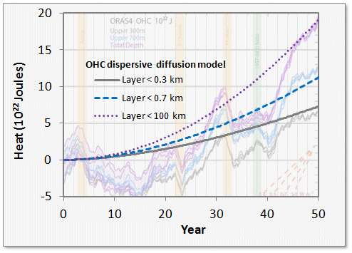Figure 2 : Thermal Dispersive Diffusion Model applied to the OHC data

Another view of the OHC includes the thermal mass of the non-ocean regions (see Figure 3). This data appears smoothed in comparison to the raw data of Figure 2.

Figure 3 :  Alternate view of growing ocean heat content. This also includes non-ocean.

In the latter figure, the agreement with the uncertainty-quantified theory is more striking. A single parameter, Hansen's effective diffusion coefficient D, along with the inferred external thermal forcing function is able to reproduce the temporal profile accurately.

The strength of this modeling approach is to lean on the maximum entropy principle to fill in the missing gaps where the variability in the numbers are uncertain.  In this case, the diffusion and ocean depths hold the uncertainty, and we use first-order phyiscs to do the rest.

Sanity Check

The following is a sanity check for the above formulation; providing essentially a homework assignment that a physics professor would hand out in class.

An application of Fick’’s Law is to approximate the amount of material that has diffused (with thermal diffusion coefficient D) at least a certain distance, x, over a time duration, t, by

$$ e^{\frac{-x}{\sqrt{Dt}}}= \frac{Q}{Q_0}$$

• For greater than 300 meters, Q/Q_0 is 13.5/20 read from Figure 1.
• For greater than 700 meters, Q/Q_0 is 7.5/20

Where Q_0=20 is the baseline for the total heat measured over all depths (i.e. between x=0 and x=infinite depth) reached at the current time. No heat will diffuse to infinite depths so at that point Q/Q_0 is 0/20.

First, we can check to see how close the value of L=sqrt(Dt) scales, by fitting the Q/Q_0 ratio at each depth..

• For x=300 meters, we get L=763
• For x=700 meters, we get L=713

These two are close enough to maintaining invariance that the Fick’’s law scaling relation holds and we can infer that the flow is by an effective diffusion, just as was surmised by Hansen et al in 1981.

We then use an average elapsed diffusion time of t=40 years and assume an average diffusion depth of 740, and D comes out to 4.5 cm^2/s.

Hansen in 1981 [2] used an estimated value of diffusion of 1 cm^2/s, which is within an order of magnitude of 4.5 cm^2/s

This is a scratch attempt at an approximate solution to the more general solution, which is the equivalent of generating an impulse function in the past and watching that evolve. The general solution which we formulated earlier involves a modulated forcing function and we compute the convolution against the thermal impulse response (i.e. Green’s function) and compare that against Figure 1 and Figure 2, and the full temporal profile.

Discussion

Reading Hansen and looking at the BTK paper’s results, we should note that nothing looks out of the ordinary for the OHC trending if we compare it to what conventional thermal physics would predict. The total heat absorbed by the ocean is within  range of that expected by a 3C doubling sensitivity. BTK has done the important step in determining the amount of total heat absorbed, which allows us to estimate the effective diffusion coefficient by evaluating how the heat contents modulate with depth.We add a maximum uncertainty modifier to the coefficient to model the disorder in diffusivity (some of it eddy diffusivity, some vertical, etc) and that allows us to match the temporal profile accurately.



References

[1]

M. A. Balmaseda, K. E. Trenberth, and E. Källén, “Distinctive climate signals in reanalysis of global ocean heat content,” Geophysical Research Letters, 2013.

[2]

J. Hansen, D. Johnson, A. Lacis, S. Lebedeff, P. Lee, D. Rind, and G. Russell, “Climate impact of increasing atmospheric carbon dioxide,” Science, vol. 213 (4511), pp. 957–966.
http://pubs.giss.nasa.gov/docs/1981/1981_Hansen_etal.pdf

 EDITED 

More data from the NOAA site using the same fit. Levitus et al [3] apply an alternative characterization to the above. I apply the same model as dashed green line.

Figure 4 : From the NOAA site, with the same model
http://www.nodc.noaa.gov/OC5/3M_HEAT_CONTENT/

And here is a plot of OHC using the effective forcing described by Hansen [4]. Instead of using a ramp forcing function which gives the analytical result of Figure 2, a realistic forcing (which takes into account perturbations due to volcanic events) is numerically convolved with the diffusive response function, I(t).

 Figure 5: Numerical convolution of effective forcing (lower left) is convolved with the diffusive transfer function to give the response (upper right).  The three curves are < 300 m,  < 700 m, and < 2000 m.

Note that the volcanic disturbances are clearly visible in the response, although they do not show as sharp a transient decrease after the events, perhaps half of what Figure 1 shows. The suppression due to the 1997-1998 El Nino is also not observable, but that of course is not a effective forcing and so won't appear.

[3]

S. Levitus, J. Antonov, T. Boyer, O. Baranova, H. Garcia, R. Locarnini, A. Mishonov, J. Reagan, D. Seidov, and E. Yarosh, “World ocean heat content and thermosteric sea level change (0–2000 m), 1955–2010,” Geophysical Research Letters, vol. 39, no. 10, 2012.

[4]

J. Hansen, M. Sato, P. Kharecha, and K. von Schuckmann, “Earth’s energy imbalance and implications,” Atmospheric Chemistry and Physics, vol. 11, no. 24, pp. 13421–13449, Dec. 2011.

Ocean map of depths