Stochastic analysis of log sensitivity to CO2

Often both skeptics and non-skeptics of AGW will suggest that climate models and their simulations are becoming too unwieldy to handle.  Stochastic models of the climate are always an option to consider, as Marston points out in his paper "Looking for new problems to solve? Consider the climate", where he recommended to

"look at the sort of question a statistical description of the climate system would be expected to answer" [5] . 

It is no wonder that applying stochasticity is one of the grand challenges in science. In the past few years, DARPA put together a list of 23 mathematical challenges inspired by Hilbert's original list. Several of them feature large scale problems which would benefit from the stochastic angle that both Marston and David Mumford [4] have recommended:

• Mathematical Challenge 3: Capture and Harness Stochasticity in Nature
  Address David Mumford’s call for new mathematics for the 21st century. Develop methods that capture persistence in stochastic environments.  
• Mathematical Challenge 4: 21st Century Fluids Classical fluid dynamics and the Navier-Stokes Equation were extraordinarily successful in obtaining quantitative understanding of shock waves, turbulence and solitons, but new methods are needed to tackle complex fluids such as foams, suspensions, gels and liquid crystals.
• Mathematical Challenge 7: Occam’s Razor in Many Dimensions
  As data collection increases can we “do more with less” by finding lower bounds for sensing complexity in systems? This is related to questions about entropy maximization algorithms.
• Mathematical Challenge 20: Computation at Scale
  How can we develop asymptotics for a world with massively many degrees of freedom?

The common theme is one of reducing complexity, which is often at odds with the mindset of those convinced that only more detailed computations of complex models will accurately represent a system.

A representative phenomena of what stochastic processes are all about is the carbon cycle and the sequestering of CO2. Much work has gone into developing box models with various pathways leading to sequestering of industrial CO2. The response curve according to the BERN model [7] is series of damped exponentials showing the long term sequestering. Yet, by a more direct statistical interpretation of what is involved in the process of CO2 sequestration, we can model the adjustment time of CO2 decay by a dispersive diffusional model derived via maximum entropy principles.

$$ I(t) = \frac{1}{1+\sqrt{t/\tau}} $$

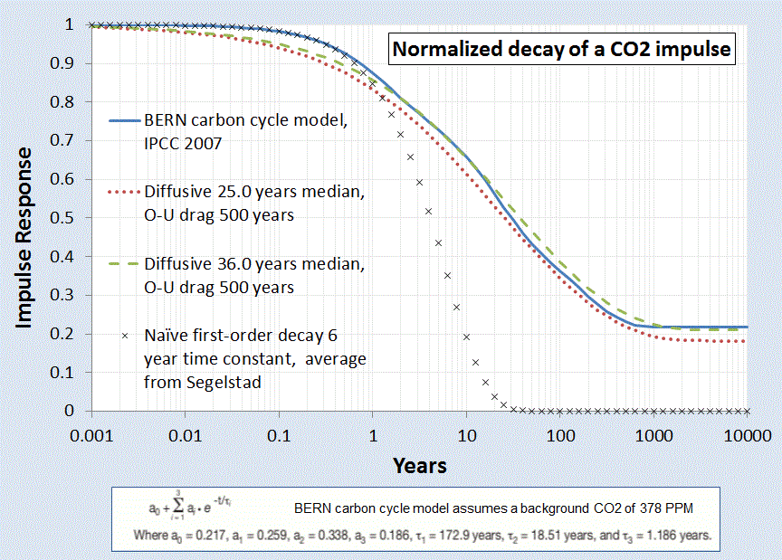Figure 1 : Impulse response of atmospheric CO2 concentration due to excess carbon emission.

A main tenet of the AGW theory presupposes the evolution of excess CO2. The essential carbon-cycle physics says that the changing CO2 is naturally governed by a base level which changes with ambient temperature, but with an additional impulse response governed by a carbon stimulus, either natural (volcano) or artificial (man-made carbon). The latter process is described by a convolution, one of the bread and butter techniques of climate scientists:

$$CO_2(t,T) = CO_2(0,T) + \kappa \int_0^t C(\tau) I(t-\tau) d\tau $$

With the impulse response of Figure 1 convolved against the historical carbon outputs as archived at the CO2 Information Analysis Center, it matches the measured CO2 from the KNMI Climate Explorer with the following agreement:

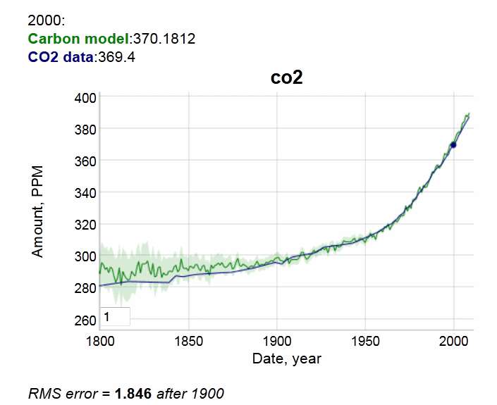Figure 2 : CO2 impulse response convolution

The match to the CO2 measurements is very good after the year 1900. No inexplicable loss of carbon to be seen. This is all explainable by diffusion kinetics into sequestration sites. Diffusional physics is so well understood that it is no longer arguable.

If on the other hand, you do this analysis incorrectly and use a naive damped exponential response ala Segalstad [1] and Salby [unpublished] and other contrarian climate scientists, you do end up apparently believing that half of the CO2 has gone missing. If that were indeed the case, this is what the response looks like, given the skeptics view of a short 6.5 year CO2 residence time:

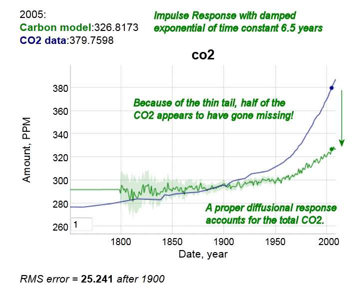Figure 3: Incorrect impulse response showing atmospheric CO2 deficit due to a short residence time.
This is clearly not observed in the data

The obvious conclusion is that if you don't do the statistical physics correctly, you end up with nonsense numbers.


Note that this does not contradict findings of the mainstream climate researchers, but it places our understanding on a potentially different footing, and one with potentially different insight.

Consider next the sensitivity of temperature to the log of atmospheric CO2. In 1863, Tyndall discovered the properties of CO2 and other gases via an experimental apparatus [3];he noticed that light radiation absorption was linear up to a point but beyond that the absorptive properties of the gas showed a diminishing effect:

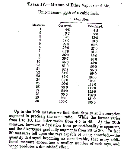Figure 4: Tyndall's description of absorption of light rays by gases [6]

The non-linear nature derives from the logarithmic sensitivity of forcing to CO2 concentration. The way to understand this is to consider differential increases of gas concentration. In the test chamber experiment, this is just a differential increase in the length of the tube. The scattering cross-section is derived as a proportional increase to how much gas is already there so it integrates as the ratio of delta increase to the cumulative length of travel of the photon:

$$ \int_{L_0}^L \frac{dX}{X} = ln(\frac{L}{L_0}) \sim ln(\Delta{[CO_2]}) $$

So as the photon travels a length of tube, it gets progressively more difficult to increase the amount of scattering, not because it isn't physically possible but because the photon has had a large probability of being intercepted already as it makes its way out of the atmosphere. That generates the logarithmic sensitivity.

Note that the lower bound of the integral has to exist to prevent a singularity in the proportional increase. To represent this another way, we can say that there is a minimum length at which the absorption cross-section occurs.


$$ \int_{0}^L \frac{dX}{X_0+X} = ln(\frac{X_0+L}{X_0}) \sim ln(1+\Delta{[CO_2]}) $$


The analogy to the test chamber is the height of the atmosphere. The excess CO2 that we emit from burning fossil fuels increases the concentration at the top of the atmosphere, and that increases the length of the travel of the outgoing IR photons, and the same logarithmic sensitivity results. This is incorrectly labeled as saturating behavior, instead of an asymptotic logarithmic behavior.

I haven't seen this derived in this specific way but the math is high-school level integral calculus. The actual model used by Lacis and other climate scientists is to configure the cross-sections by compositing the atmosphere into layers or "slabs" and then propagating the interception of photons by CO2 by differential numerical calculations. In addition, there is a broadening of the spectral lines as concentration increases, contributing to the first order result of logarithmic sensitivity.  In general the more that the infrared parts of the photonic spectrum get trapped by CO2 and H20, the higher the temperature has to be to make up for the missing propagated wavelengths while not violating the earth's strict steady-state incoming/outgoing energy balance.

To get a sense of this logarithmic climate sensitivity, the temperature response is shown to the below  right for a 3°C sensitivity to CO2 doubling, mapped against the BEST land-based temperature record. Observe that trending temperature shifts are already observed in the early 20th century.

Figure 5:  CO2 model applied to AGW via a log sensitivity and
compared against the fast rsponse of BEST land-based records.

If we choose a 2.8°C sensitivity from Hansen's 1981 paper [2] and compare the above model to Hansen's projection, one can see that we are on the right track in duplicating his analysis.

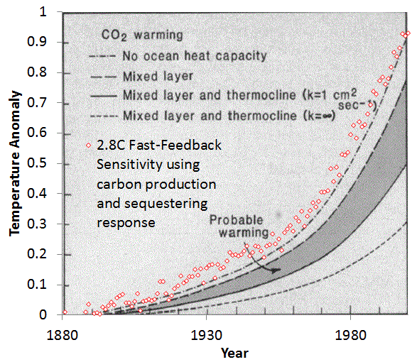Figure 6: Hansen's original model projection circa 1981 [2] and the 2.8C model used here.

Perhaps the only real departure from the model is a warming around 1940 not accounted for by CO2.  But even this is likely due to a stochastic characteristic in the form of noise riding along with the trend.. This noise could be volcanic disruptions or ocean upwelling fluctuations of a random nature,  which only requires the property that upward excursions match downward.

So if we consider the difference between the green line model and blue line data below:

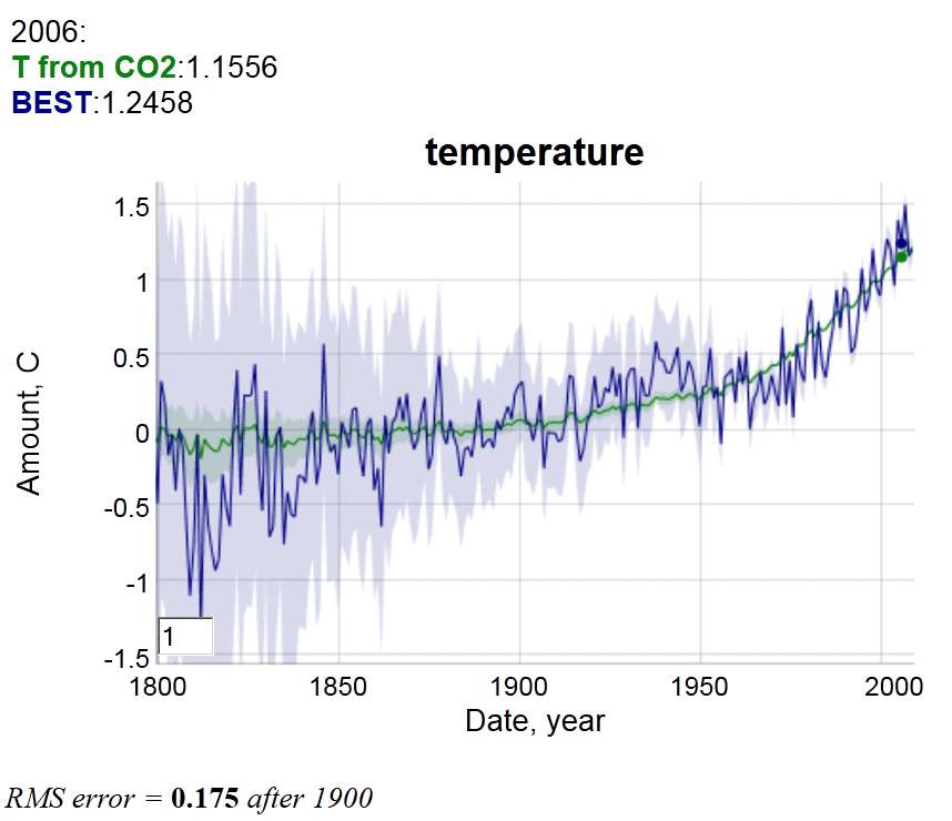Figure 7: Plot used for regression analysis.
Beyond 1900, the RMS error is less than 0.2 degrees

and take the model/data residuals over time, we get the following plot.

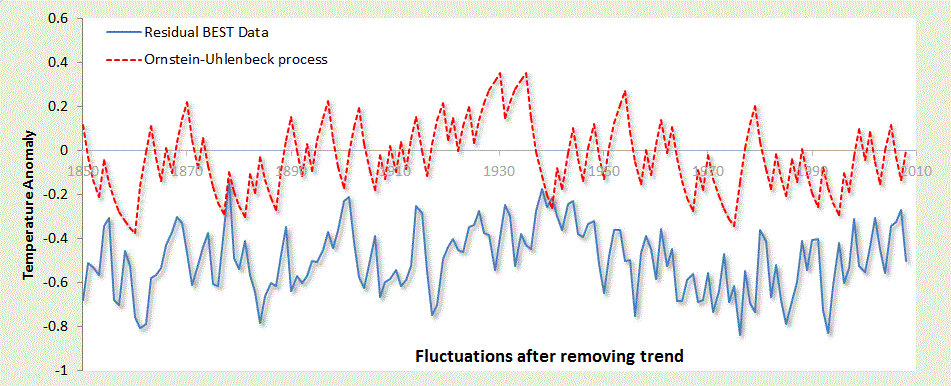Figure 8: Regression difference between log sensitivity model and BEST data 

Note that the yearly excursions never exceed about 0.2°C from the underlying trend.  The dotted line red curve above the solid blue residual curve is an Ornstein-Uhlenbeck model (red noise) of a yearly random walk with a reversion-to-the-mean drag that prevents fluctuations beyond approximately 0.2°C.  At this kind of scale and considering the Markov process which will allow short-term fluctuations in the tenths of a degree, the bump of increased temperature in the 1940's is not a rare nor completely unlikely occurrence.

A red noise model on this scale can not accommodate both the short-term fluctuations and the large upward trend of the last 50 years. That is why the CO2-assisted warming is the true culprit, as evidenced by a completely stochastic analysis.

[EDIT]
Here is a sequence of red noise time series (of approximately 0.2°C RMS excursion) placed on top of an accelerating monotonically warming temperature profile (the no-noise accelerating profile is in the lower left panel). The actual profile is shown in the lower right panel. An averaging window of 30 years is placed on the profiles to give an indication of where plateaus, pauses, and apparent cooling can occur.

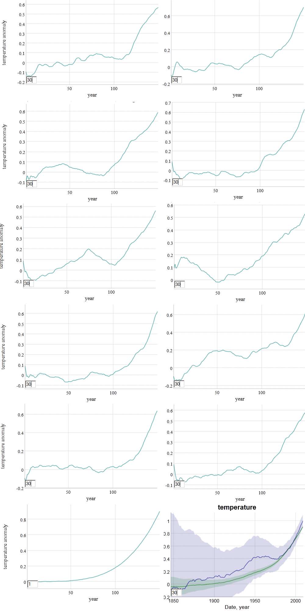Figure 9: Hypothetical red noise series placed on an accelerating warming curve.

"Noise riders" are people that look at time series and read too much into each fluctuation. The temptation to place too much emphasis on recent readings is strong but ultimately misguided. Dead reckoning models are built-in as a human intuition mechanism but don't serve us well in the face of noise.

The baseball analogy to the red noise of Figure 9 is the knuckle-ball pitcher. Being able to hit a knuckle-baller means that you have quick reflexes and an ability to suppress the dead reckoning urge.

R.A. Dickey's Cy Young Knuckleball Pitch (SOURCE)

References

[1]

T. V. Segalstad, “Carbon cycle modelling and the residence time of natural and anthropogenic atmospheric CO2,” BATE, R.(Ed., 1998): Global Warming, pp. 184–219, 1998.

[2]

J. Hansen, D. Johnson, A. Lacis, S. Lebedeff, P. Lee, D. Rind, and G. Russell, “Climate impact of increasing atmospheric carbon dioxide,” Science, 2l3, pp. 957–966.

[3]

A. A. Lacis, G. A. Schmidt, D. Rind, and R. A. Ruedy, “Atmospheric CO2: principal control knob governing Earth’s temperature,” Science, vol. 330, no. 6002, pp. 356–359, 2010.

[4]

D. Mumford, “The dawning of the age of stochasticity,” Mathematics: Frontiers and Perspectives, pp. 197–218, 2000.

[5]

B. Marston, “Looking for new problems to solve? Consider the climate,” Physics, vol. 4, p. 20, 2011.

[6] Tyndall, John, 1861. On the Absorption and Radiation of Heat by Gases and Vapours, and on the Physical Connection of Radiation, Absorption, and Conduction. 'Philosophical Magazine ser. 4, vol. 22, 169–94, 273–85.

[7] J. Golinski, “Parameters for tuning a simple carbon cycle model,” United Nations Framework Convention on Climate Change. [Online]. Available: http://unfccc.int/resource/brazil/carbon.html. [Accessed: 12-Mar-2013].