Thermal Diffusion and the Missing Heat

I have this documented already (in The Oil Conundrum) but let me put a new spin on it. What I will do is solve the heat equation with initial conditions and boundary conditions for a simple experiment. And then I will add two dimensions of Maximum Entropy priors.

The situation is measuring the temperature of a buried sensor situated at some distance below the surface after an impulse of thermal energy is applied. The physics solution to this problem is the heat kernel function which is the impulse response or Green's function for that variation of the master equation. This is pure diffusion with no convection involved (heat is not sensitive to fields, gravity or electrical, so no convection).

However the diffusion coefficient involved in the solution is not known to any degree of precision. The earthen material that the heat is diffusing through is heterogeneously disordered, and all we can really guess at that it has a mean value for the diffusion coefficient. By inferring through the maximum entropy principle, we can say that the diffusion coefficient has a PDF that is exponentially distributed with a mean value D.

We then work the original heat equation solution with this smeared version of D, and then the kernel simplifies to a exp() solution.
$$ {1\over{2\sqrt{Dt}}}e^{-x/\sqrt{Dt}} $$
But we also don't know the value of x that well and have uncertainty in its value. If we give a Maximum Entropy uncertainty in that value, then the solution simpilfies to
$$ {1\over2}{1\over{x_0+\sqrt{Dt}}} $$
where x0 is a smeared value for x.

This is a valid approximation to the solution of this particular problem and the following Figure 1 is a fit to experimental data. There are two parameters to the model, an asymptotic value that is used to extrapolate a steady state value based on the initial thermal impulse and the smearing value which generates the red line. The slightly noisy blue line is the data, and one can note the good agreement.

Figure 1: Fit of thermal dispersive diffusion model (red) to a heat impulse response (blue).

Notice the long tail on the model fit.  The far field response in this case is the probability complement of the near field impulse response. In other words, what diffuses away from the source will show up at the adjacent target. By treating the system as two slabs in this way, we can give it an intuitive feel.

By changing an effective scaled diffusion coefficient from small to large, we can change the tail substantially, see Figure 2. We call it effective because the stochastic smearing on D and Length makes it scale-free and we can longer tell if the mean in D or Length is greater. We could have a huge mean for D and a small mean for Length, or vice versa, but we could not distinguish between the cases, unless we have measurements at more locations.

Figure 2 : Impulse response with increasing diffusion coefficient top to bottom.
The term x represents time, not position .

In practice, we won't have a heat impulse as a stimulus. A much more common situation involves a step input for heat. The unit step response is the integral of the scaled impulse response

The integral shows how the heat sink target transiently draws heat from the source.  If the effective diffusion coefficient is very small, an outlet for heat dispersal does not exist and the temperature will continue to rise. If the diffusion coefficient is zero, then the temperature will increase linearly with time, t (again this is without a radiative response to provide an outlet). 

Figure 3 : Unit step response of dispersed thermal diffusion. The smaller the effective
thermal diffusion coefficient, the longer the heat can stay near the source.

Eventually the response will attain a square root growth law, indicative of a Fick's law regime of what is often referred to as parabolic growth (somewhat of a misnomer).  The larger the diffusion coefficient, the more that the response will diverge from the linear growth. All this means is that the heat is dispersively diffusing to the heat sink.

Application to AGW

This has implications for the "heat in the pipeline" scenario of increasing levels of greenhouse gases and the expected warming of the planet.  Since the heat content of the oceans are about 1200 times that of the atmosphere, it is expected that a significant portion of the heat will enter the oceans, where the large volume of water will act as a heat sink.  This heat becomes hard to detect because of the ocean's large heat capacity; and it will take time for the climate researchers to integrate the measurements before they can conclusively demonstrate that diffusion path.

In the meantime, the lower atmospheric temperature may not change as much as it could, because the GHG heat gets diverted to the oceans.  The heat is therefore "in the pipeline", with the ocean acting as a buffer, capturing the heat that would immediately appear in the atmosphere in the absence of such a large heat sink.  The practical evidence for this is a slowing of the atmospheric temperature rise, in accordance with the slower sqrt(t) rise than the linear t.   However, this can only go on so long, and when the ocean's heat sink provides a smaller temperature difference than the atmosphere, the excess heat will cause a more immediate temperature rise nearer the source, instead of being spread around.

In terms of AGW, whenever the global temperature measurements start to show divergence from the model, it is likely due to the ocean's heat capacity.   Like the atmospheric CO2, the excess heat is not "missing" but merely spread around.

EDIT:
The contents of this post are discussed on The Missing Heat isn't Missing at all.

I mentioned in comments that the analogy is very close to sizing a heat sink for your computer’s CPU. The heat sink works up to a point, then the fan takes over to dissipate that buffered heat via the fins. The problem is that the planet does not have a fan nor fins, but it does have an ocean as a sink. The excess heat then has nowhere left to go. Eventually the heat flow reaches a steady state, and the pipelining or buffering fails to dissipate the excess heat.


What's fittingly apropos is the unification of the two "missing" cases of climate science.

1. The "missing" CO2. Skeptics often complain about the missing CO2 in atmospheric measurements from that anticipated based on fossil fuel emissions. About 40% was missing by most accounts. This lead to confusion between the ideas of residence times versus adjustment times of atmospheric CO2. As it turns out, a simple model of CO2 diffusing to sequestering sites accurately represented the long adjustment times and the diffusion tails account for the missing 40%. I derived this phenomenon using diffusion of trace molecules, while most climate scientists apply a range of time constants that approximate diffusion.

2. The "missing" heat. Concerns also arise about missing heat based on measurements of the average global temperature. When a TCR/ECS* ratio of 0.56 is asserted, 44% of the heat is missing. This leads to confusion about where the heat is in the pipeline. As it turns out, a simple model of thermal energy diffusing to deeper ocean sites may account for the missing 44%. In this post, I derived this using a master heat equation and uncertainty in the parameters. Isaac Held uses a different approach based on time constants.

So that is the basic idea behind modeling the missing quantities of CO2 and of heat -- just apply a mechanism of dispersed diffusion. For CO2, this is the Fokker-Planck equation and for temperature, the heat equation. By applying diffusion principles, the solution arguably comes out much more cleanly and it will lead to better intuition as to the actual physics behind the observed behaviors.


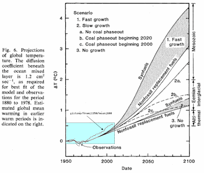
I was alerted to this paper by Hansen et al (1985) which uses a box diffusion model. Hansen’s Figure 2 looks just like my Figure 3 above. This bends over just like Hansen’s does due to the diffusive square root of time dependence. When superimposed, it is not quite as strong a bend as shown in Figure 4 below.

Figure 4: Comparison against Hansen's model of diffusion

This missing heat is now clarified in my mind. In the paper Hansen calls it “unrealized warming”, which is heat entering into the ocean without raising the climate temperature substantially.

EDIT:
The following figure is a guide to the eye which explains the role of the ocean in short- and long-term thermal diffusion, i.e. transient climate response. The data from BEST illustrates the atmospheric-land temperatures, which are part of the fast response to the GHG forcing function. While the GISTEMP temperature data reflects more of the ocean's slow response.

Figure 5: Transient Climate Response explanation

Figure 6: Hansen's original projection of transient climate sensitivity plotted against the GISTEMP data,
which factors in ocean surface temperatures.

*
TCR = Transient Climate Response
ECS = Equilibrium Climate Sensitivity

---

Added:

"Somewhere around 23 x 10^22 Joules of energy over the past 40 years has gone into the top 2000m of the ocean due to the Earth’s energy imbalance "

That is an amazing number. If one assumes an energy imbalance of 1 watt/m^2, and integrate this over 40 years and over the areal cross-section of the earth, that accounts for 16 x 10^22 joules.

The excess energy is going somewhere and it doesn't always have to be reflected in an atmospheric temperature rise.

To make an analogy consider the following scenario.

Lots of people understand how the heat sink works that is attached to the CPU inside a PC. What the sink does is combat the temperature rise caused by the electrical current being injected into the chip. That number multiplied by the supply voltage gives a power input specified in watts. Given a large enough attached heat sink, the power gets dissipated to a much large volume before it gets a chance to translate quickly to a temperature rise inside the chip. Conceivably, with a large enough thermal conductance and a large enough mass for the heat sink, and an efficient way to transfer the heat from the chip to the sink, the process could defer the temperature rise to a great extent. That is an example of a transient thermal effect.

The same thing is happening to the earth, to an extent that we know must occur but with some uncertainty based on the exact geometry and thermal diffusivity of the ocean and the ocean/atmospheric interface. The ocean is the heat sink and the atmosphere is the chip. The difference is that much of the input power is going directly into the ocean, and it is getting diffused into the depths. The atmosphere doesn't have to bear the brunt of the forcing function until the ocean starts to equilibrate with the atmosphere's temperature. This of course will take a long time based on what we know about temporal thermal transients and the Fickian response of temperature due to a stimulus.

The belief in Chaos

The Chief says :

“Nothing just happens randomly in the Earth climate system. Randomness – or stochasticity – is merely a statistical approach to things you haven’t understood yet. ”

One of the unsung achievements in physics, in comparison to the imagination-capturing aspects of relativity and quantum mechanics, is statistical mechanics. This will scale at many levels -- originally intended to bridge the gap between the microscopic theory and macroscopic measurements, such as with the Planck response, scientists have provided statistical explanations to large coarse-grained behaviors as well (wind, ocean wave mechanics, etc). It's not that we don't understand the chaotic underpinnings, more like that we don't always need to, due the near-universal utility of the Boltzmann partition function (see the discussion on the Thermodynamics Climate Etc thread).

Many scientists consider pawning off difficulties to "Chaos" as a common crutch. This is not my original thought, as it is discussed at depth in Science of Chaos or Chaos in Science" by Bricmont. The issue with chaos theories is that they still have to obey some fundamental ideas of energy balance and conservation laws. Since stochastic approaches deal with probabilities, one rarely experiences problems with the fundamental bookkeeping. The basic idea with probability, that it has to integrate to unity probability, making it a slick tool for basic reasoning. That is why I like to use it so much for my own basic understanding of climate science (and all sorts of other things), but unfortunately leads to heated disagreements to the chaos fans and non-linear purists, such as David Young and Chief Hydrologist. They are representative of the opposite side of the debate.

You notice this when Chief states the importance of chaos theory:

"You should try to understand and accept that – along with the reality that my view has considerable support in the scientific literature. You should accept also that I am the future and you are the past.

I think they sould teach the 3 great ideas in 20th centruy physics – relativity, quantum mechanics and chaos theory. They are such fun."

There are only 4 fundamental forces in the universe, gravity, electromagnetism, and the strong and weak nuclear forces. For energy balance of the earth, all that matters is the electromagnetic force, as that is the predominant way that the earth exchanges energy with the rest of the universe.

The 33 degree C warming temperature differential from the earth's gray-body default needs to be completely explained by a photonic mechanism.

The suggestion is that clouds could change the climate. Unfortunately this points it in the incorrect direction of explaining the 33C difference. Water vapor, when not condensed into droplets, acts as a strong GHG and likely does cause a significant fraction of the 33C rise. But when the water vapor starts condensing into droplets and thus forming clouds, the EM radiation begins to partially reflect the incoming radiation, and thus the sun providing even less heat to the earth. So obviously there is a push-pull effect to raising water vapor concentrations in the atmosphere.

Chief is daring us with his statement that "I am the future and you are the past". He evidently thinks that clouds are the feedback that will not be understood unless we drop down to chaos considerations. In other words, that any type of careful statistical considerations of the warming impact of increasing water vapor concentrations with the cooling impact of cloud albedo, will not be explainable unless a full dynamical model is attempted and done correctly.


The divide is between whether one believes as Chief does, that the vague "chaos theory", which is really short-hand for doing a complete dynamical calculation of everything, no exceptions, is the answer. Or is the answer one of energy balance and statistical considerations? I lean toward the latter, along with the great majority of climate scientists, as Andrew Lacis described a while ago here and in his comments. The full dynamics, as Lacis explained is useful for understanding natural variability, and for practical applications such as weather prediction. But it is not the bottom-line, as chaotic natural variability always has to obey the energy balance constraints. And the only practical way to do that is by considering a statistical view.

---

The bottom-line is that I chuckle at much of the discussion of chaos and non-linearity when it comes to try to understand various natural phenomenon. The classic case is the simplest model of growth described by the logistic differential equation. This is a non-linear equation with a solution described by the so-called logistic function. Huge amounts of work have gone into modeling growth using the logistic equation because of the appearance of an S-shaped curve in some empirical observations. (when it is a logistic difference equation, chaotic solutions result but we will ignore that for this discussion)

Alas, there are trivial ways of deriving the same logistic function without having to assume non-linearity or chaos; instead one only has to assume disorder in the growth parameters and in the growth region. The derivation takes a few lines of math (see the TOC).

Once one considers this picture, the logistic function arguably has a more pragmatic foundation based on stochastics than on non-linear determinism.

That is the essential problem of invoking chaos, in that it precludes (or at least masks) considerations of the much more mundane characteristics of the system. The mundane is that all natural behaviors are smeared out by differences in material properties/characteristics, variation in geometrical considerations, and in thermalization contributing to entropy.

The issue is that obsessives such as the Chief and others think that chaos is the hammer and that they can apply it to every problem that appears to look like a nail.

Certainly, I can easily understand how the disorder in a large system can occasionally trigger tipping points or lead to stochastic resonances, but these are not revealed by analysis of any governing chaotic equations. They simply result from the disorder allowing behaviors to penetrate a wider volume of the state space. When these tickle the right positive feedback modes of the system, then we can observe some of the larger fluctuations. The end result is that the decadal oscillations are of the order of a tenths of degrees in global average temperature.

Of course I am not wedded to this thesis, just that it is a pragmatic result of stochastic and uncertainty considerations that I and a number other people are interested in.

---

This is reproduced from a comment I made to Climate Etc:

I am glad that Myrrh posted this bit of pseudoscience.

As I said earlier (when I thought that this thread was winding down) the actual pseudoscience is in the crackpot theories that commenters submit to this site. There is a huge amount of projection that goes on amongst the skeptical readership -- the projection is in the framing of their own scientific inadequacies onto the qualified scientists trying to understand and quantify the climate system.

Projection is a devious rhetorical strategy. It is an offensive as opposed to defensive approach. It catapults the propaganda from one of doubt on the skeptical side, to an apparent uncertainty on the mainstream science side. This adds FUD to the debate. As in politics, by attacking the strong points of your opponents argument, you can actually make him look weaker. Everyone realizes how effective this is whenever the audience does not have the ability to discriminate nonsense from objective fact.

The key to projection is to make sure that the confidence game is played out according to script amongst the participants, both those in on the game and those unaware of what is happening. The shills in on the game have it easy -- they just have to remain silent, as it appears that no comment is condoning the arguments. The marks are the readership that gets suckered into the pseudoscience arguments, and are not sophisticated enough to be aware of the deception.

The antidote to this is to not remain silent. Call these confidence tricksters, including Myrrh, out on their game. Do it every time, because a sucker is born every minute. On the street corner, the 3-Card Monte hucksters will just move to another corner when they get called on it. Fortunately, there is no place for the tricksters to relocate on this site.

Ultimately, science has the advantage, and as the objective of Climate Etc is to work out uncertainty objectively, not by confidence games, you all should know about the way to proceed. Sorry if this bursts any bubbles, but when it comes to an aggressively nonsensical argument as that relayed by Myrrh, someone has to keep score.

Then you have a kook like StephanTheDenier, where he actually tries a thinly veiled psychological threat against me, by saying ("The souls of hose 600 people that did freeze to death in winter coldness, will haunt you in your sleep…"). What can I say but that threats are even more preposterous than projecting via lame theories.

----------
And in reading Bart's rebuttal, I just want to add:

Outside of a sled dog, an igloo is an Eskimo's best friend.
Inside of a sled dog, it's too cramped to sleep.

Wave Energy Spectrum

Ocean waves are just as disordered as the wind. We may not notice this because the scale of waves is usually smaller. In practice, the wind energy distribution relates to an open water wave energy distribution via similar maximum entropy disorder considerations. The following derivation assumes a deep enough water such that troughs do not touch bottom

First, we make a maximum entropy estimation of the energy of a one-dimensional propagating wave driven by a prevailing wind direction. The mean energy of the wave is related to the wave height by the square of the height, H. This makes sense because a taller wave needs a broader base to support that height, leading to a scaled pseudo-triangular shape, as shown in Figure 1 below.

Figure 1: Total energy in a directed wave goes as the square of the height, and the macroscopic fluid
properties suggest that it scales to size. This leads to a dispersive form for the wave size distribution

 Since the area of such a scaled triangle goes as H^2, the MaxEnt cumulative probability is:

$$ P(H) = e^{-a H^2} $$

where a is related to the mean energy of an ensemble of waves. This relationship is empirically observed from measurements of ocean wave heights over a sufficient time period. However, we can proceed further and try to derive the dispersion results of wave frequency, which is the very common oceanography measure. So we consider -- based on the energy stored in a specific wave -- the time, t, it will take to drop a height, H, by the Newton's law relation:

$$ t^2 \sim H $$

and since t goes as 1/f, then we can create a new PDF from the height cumulative as follows:

$$ p(f) df = \frac{dP(H)}{dH} \frac{dH}{df} df $$

where

$$ H \sim \frac{1}{f^2} $$

$$ \frac{dH}{df} \sim -\frac{1}{f^3} $$

then

$$ p(f) \sim \frac{1}{f^5} e^{-\frac{c}{f^4}} $$

which is just the Pierson-Moskowitz wave spectra that oceanographers have observed for years (developed first in 1964, variations of this include the Bretschneider and ITTC wave spectra) .

This concise derivation works well despite the correct path of calculating an auto-correlation from p(f) and then deriving a power spectrum from the Fourier Transform of p(f). Yet this convenient shortcut remains useful in understanding the simple physics and probabilities involved.



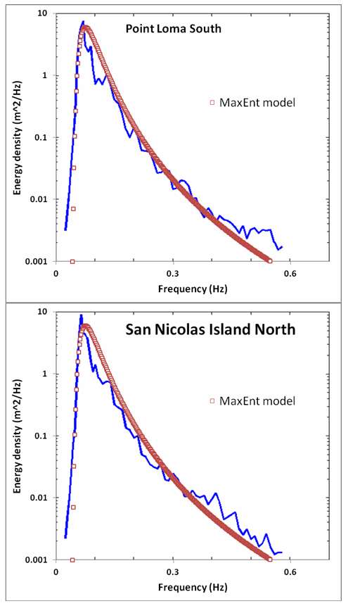
As we have an interest in using this derived form for an actual potential application, we can seek out public-access stations to obtain and evaluate some real data. The following Figure 2 is data pulled from the first region I accessed -- a pair of measuring stations located off the coast of San Diego. The default data selector picked the first day of this year, 1/1/2012 and the station server provided an averaged wave spectra for the entire day.  The red points correspond to best fits from the derived MaxEnt algorithm to the blue data set.

Figure 2: Wave energy spectra from two sites off of the San Diego coastal region.
The Maximum Entropy estimate is in red.

To explore the dataset, here is a link to the interactive page :
http://cdip.ucsd.edu/?nav=historic&sub=data&units=metric&tz=UTC&pub=public&map_stati=1,2,3&stn=167&stream=p1&xyrmo=201201&xitem=product25

Like the wind energy spectrum, the wave spectrum derives simply from maximum entropy conditions.

Refs
Introduction to physical oceanography, RH Stewart