Context/Earth

Please refer to my new Wordpress blog Context/Earth for future posts.

Wordpress has better commenting options such as provisions for pictures and charts.

The scope of the blog is also more comprehensive, as it will include all environmental and energy topics tied together in a semantic web framework. 

Onward and upward as they say.

Expansion of atmosphere and ocean

This is a short tutorial together with some observational evidence explaining how the atmosphere and ocean is expanding measurably in the face of global warming.

Ocean thermal expansion

The ocean absorbs heat per area according to its heat capacity

$$ \Delta E = C_p \cdot \Delta T \cdot {Depth}$$

The linear coefficient of thermal expansion is assumed constant over a temperature range. Multiplying this over a depth:

$$ \Delta Z = \epsilon \cdot \Delta T \cdot Depth $$
But now we can substitute the total energy gained from the first equation:
$$ \Delta Z = \epsilon \frac{\Delta E}{C_p} $$
Assume that the linear coefficient of thermal expansion is 0.000207 per °C, and specific heat capacity is 4,000,000 J/m^3/°C.

If an excess forcing of 0.6 W/m^2 occurs over one year (see the OHC model), then the increase in the level of the ocean is

0.000207  * 0.6*(365*24*60*60) / 4,000,000 = 0.98 mm

This is called the steric sea-level rise, and it is just one component of the sea-level rise over time (the others have to do with melting ice). From the figure below, one can see that the thermal rise is close to 1mm/year over the last decade.

The red line shows the thermal expansion from the ocean heating. Thermal rise is 1 mm/year over the 3 mm/year total sea-level rise.

Atmosphere thermal expansion

The trick here is to infer the atmosphere expansion by looking at an equal pressure point as a function of altitude (a geopotential height isobar) and determine how much that point has increased over time.  I was able to find one piece of data from The Weather Channel's senior meteorologist Stu Ostro.

The geopotential height anomaly is shown below for the 500 mb (1/2 atmosphere)

Geopotential height anomaly @ 500 mb plotted alongside global temperature anomaly.

In absolute terms it is charted as follows:

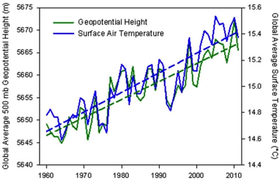Global average geopotential height @ 500 mb plotted alongside global temperature.
http://icons-ak.wxug.com/graphics/earthweek/geopotential-height-and-air-temperature.png

To understand how the altitude has changed, consider the classical barometric formula:
$$ P(H) = P_0 e^{-mgH/RT} $$

We take the point at which we reached 1/2 the STP of 1 atmosphere at sea-level:

$$ P(H)/P_0 = 0.5 = e^{-mgH/RT} $$

or
$$ H = RT/mg \cdot ln(2) $$
Assuming the average molecular weight of the atmospheric gas constituents does not change, the change in altitude (H) should be related to the change in temperature (T) by:
$$ \Delta H = R \Delta T / mg \cdot ln(2) $$
or
$$ \frac{ \Delta H}{\Delta T} =  \frac{R}{mg} ln(2) $$
For R = 8314, m=29, and g=9.8, the slope should be 29.25 *ln(2) = 20.3 m/°C.

From the linear regression agreement between the two, we get a value of 25.7 m/°C.

Linear regression between the geopotential height change and temperature change

Why is this geopotential height change about 26% higher than it should be from the theoretical value considering that the height should track the temperature according to the barometric formula?

If we use the polytropic approximation (equation 1 in the barometric formula), the altitudinal difference between the low temperature and high temperature 500 mb pressure values remains the same as when we use the classic exponential damped barometric formula:

If we apply the polytropic barometric formula instead of the exponential, we still show a real height change that is higher than theoretically predicted by ~25% at the 500 mb isobar.

This discrepancy could be due to measurement error, as the readings are taken by weather balloons and the accuracy could have drifted over the years.

It is also possible that the composition of the atmosphere could have changed slightly at altitude. What happens if the moisture increased slightly? This shouldn't make much difference.

Most likely is the possibility that the baseline sea-level pressure has changed, which shifted the 500 mbar point artificially. See http://www.ipcc.ch/publications_and_data/ar4/wg1/en/ch10s10-3-2-4.html.

"10.3.2.4 Sea Level Pressure and Atmospheric Circulation

As a basic component of the mean atmospheric circulations and weather patterns, projections of the mean sea level pressure for the medium scenario A1B are considered. Seasonal mean changes for DJF and JJA are shown in Figure 10.9 (matching results in Wang and Swail, 2006b). Sea level pressure differences show decreases at high latitudes in both seasons in both hemispheres. The compensating increases are predominantly over the mid-latitude and subtropical ocean regions, extending across South America, Australia and southern Asia in JJA, and the Mediterranean in DJF. Many of these increases are consistent across the models. This pattern of change, discussed further in Section 10.3.5.3, has been linked to an expansion of the Hadley Circulation and a poleward shift of the mid-latitude storm tracks (Yin, 2005). This helps explain, in part, the increases in precipitation at high latitudes and decreases in the subtropics and parts of the mid-latitudes. Further analysis of the regional details of these changes is given in Chapter 11. The pattern of pressure change implies increased westerly flows across the western parts of the continents. These contribute to increases in mean precipitation (Figure 10.9) and increased precipitation intensity (Meehl et al., 2005a). "

I will have to figure out the mean sea-level pressure change over this time period to verify this hypothesis.

The following recent research article looks into the shifts in geopotential height over shorter time durations:

[1]

Y. Y. Hafez and M. Almazroui, “The Role Played by Blocking Systems over Europe in Abnormal Weather over Kingdom of Saudi Arabia in Summer 2010,” Advances in Meteorology, vol. 2013, p. 20, 2013.

 

                   ADDED  7/8/2013                

One possibility for the larger-than-expected altitude change is that the average lapse rate has changed slightly.  We can use the lapse rate variation of the barometric formula, and perturb the lapse rate, L, around its average value:

$$ P(H) = P(0) (1- \frac{LH}{T_0})^{\frac{gm}{LR}} $$

Granted, the error bars on this calculation are significant but we can see how subtle the effect is.

Sea-level pressure, P(0) = 1013.25 mb
Gas constant,  R = 8.31446 J/K/mol
Earth's gravity, g = 9.807 m/s^2
Avg molecular weight, m = 0.02896 kg/m

In 1960, the temperature was about 14.65°C and 500 mb altitude was 5647 m.
In 2010, the temperature was about 15.4°C and 500 mb altitude was 5667 m.

All we need to do is invert the P(H) formula for each pair of values, modifying L slightly.

If we select a lapse rate, L, for 1960 of 0.0051°C/m, we calculate H = 5647.9m for P(H)=500 mb.
If we select a lapse rate, L, for 2010 of 0.0050°C/m, we calculate H = 5668.4m for P(H)=500 mb.

The difference in the two altitudes for a change in L of -0.0001°C/m is 20.5m, about what the geopotential height chart shows.

If we leave the L at 0.0051°C/m for both 1960 and 2010, the difference of the 500mb altitudes is only 14.7m.

To the extent that we can trust the numbers on the charts from Ostro, the change in geopotential height is suggesting a feedback effect in the lapse rate due to global warming.  The lapse rate is decreasing over time, which implies that the heat capacity of the atmosphere is increasing (likely due to higher specific humidity), thereby buffering changes in temperature with altitude.

This means that a given temperature increase at a particular altitude (where the CO2 IR window can achieve a radiative balance) will be reflected as a scale-modified temperature at sea level

In 1960, the temperature difference at 500mb altitude is 0.0051°C/m * 5647.9m = 28.80°C
In 2010, the temperature difference at 500mb altitude is 0.0050°C/m * 5668.4m = 28.34°C

The difference at sea-level from the chart is 15.4°C-14.65°C = 0.75°C whereas the difference at the 500mb altitude assuming the modified lapse rate is 0.75°C - 0.46°C = 0.29°C.  If the lapse rate didn't change then this sea-level difference would maintain at a constant atmospheric pressure isobar in altitude.

For implications in the interpretation, see page 24 of National Research Council Panel on Climate Change Feedbacks (2003). Understanding climate change feedbacks : National Academies Press. ISBN 978-0-309-09072-8.  They caution that the measurements require some precision, otherwise the errors can multiply due to the differences between two large numbers.

Characterization of Battery Charging and Discharging

I had the good fortune of taking a week long Society of Automotive Engineers (SAE) Academy class on hybrid/electric vehicles. The take-home message behind HEV and EV technology is to remember that a quality battery plus optimizing the management of battery cycling remain the keys to success.   That is not surprising --  we all know that gasoline has long been "king", and since current battery technology has nowhere near the energy density of gasoline, the battery has turned into a "diva".  In other words, it will perform as long as it is in charge (so to speak) and the battery is well maintained.

I can report that much class time was devoted to the electrochemistry of Lithium-ion batteries. Lithium is an ideal elemental material due to its position in the upper left-hand corner of the periodic table -- in other words a very lightweight material with a potentially high energy density.

What was surprising to me was the sparseness of detailed characterization of the material properties. One instructor stated that the lack of measured diffusion properties for battery cell specifications was a pet peeve of his.  Having these properties at hand allows a design engineer to better model the charging and discharging characteristics of the battery, and thus to perhaps to develop better battery management schemes. Coming from the semiconductor world, it is almost unheard of to do design without adequate device characteristics such as mobility and diffusivity.

From my perspective, this is not necessarily bad. Any time I see an anomalous behavior or missing piece, it opens the possibility I can fill a modeling niche.

Introduction

Modern rechargeable battery technology still relies on the principles of electro-chemistry and a reversible process, which hasn’t changed in fundamental terms since the first lead-acid battery came to market in the early 1900’s. What has changed is the combination of materials that make a low-cost, lightweight, and energy-efficient battery which will serve the needs of demanding applications such as electric and hybrid-electric vehicles (EV/HEV).

As energy efficient operation is dependent on the properties of the materials being combined, it is well understood that characterizing the materials is important to advancing the state-of-the-art (and in increasing EV acceptance).

Of vital importance is the characterization of diffusion in the electrode materials, as that is the rate-limiting factor in determining the absolute charging and discharging speed of the material-specific battery technology. Unfortunately, because of the competitive nature of battery producers, many of the characteristics are well-guarded and treated as trade secrets. For example, it is very rare to find diffusion coefficient characteristics on commercial battery specification sheets, even though this kind of information is vital for optimizing battery management schemes [7].

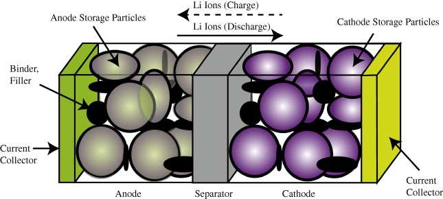
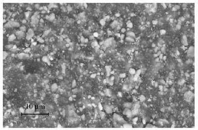
In comparison to the relatively simple diffusional mechanisms of silicon oxide growth, the engineered structure of well-designed battery cell presents a significant constraint to the diffusional behavior. In Figure 1 below we show a schematic of a single lithium-ion cell and the storage particles that charge and discharge. The disordered nature of the storage particles in Figure 2 is often described by what is referred to as a tortuosity measure.

Figure 1: Exaggerated three-dimensional view of a lithium-ion battery cell and the direction of current flow during charging and discharging

Figure 2 : Realistic view of the heavily disordered nature of the LiFePO4 storage particles [1].

The constraints on the diffusion is that it is limited in scale to that of the radius of the storage particle. The length scale is limited essentially to the values L to Lmax shown in Figure 3 below.

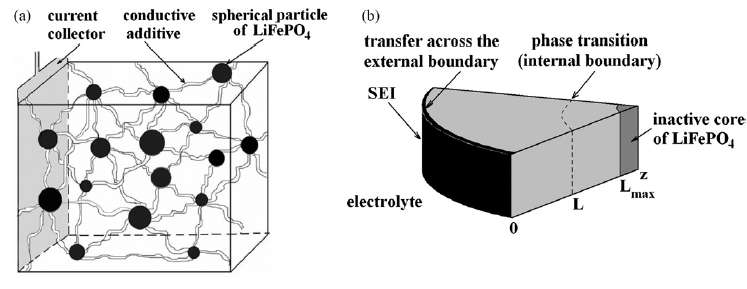Figure 3 : Diffusion of ions takes place through the radial shell of the LiFePO4 spherical particle [1]. During the discharge phase, the ions need to migrate outward through shell and through the SEI barrier before reaching the electrolyte. At this point they can contribute to current flow.

The size of the particles also varies as shown in Figure 4 below.  The two Lithium-ion materials under consideration, LiFePO4 and LiFeSO4F, have different materials properties but are structurally very similar (matrixed particles of mixed size) so that we can use a common analysis approach.  This essentially allows us to apply uncertainty in the diffusion coefficient and uncertainties in the particle size to establish a common diffusional behavior formulation.

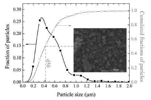Figure 4 : Particle size distribution of FeSO4F spherical granules [2]. The variation in lengths and material diffusivities opens the possibility of applying uncertainty quantification to a model of diffusive growth.

Dispersive Diffusion Analysis of Discharging

The diffusion of ions through the volume of a spherical particle does have similarity to classical regimes such as the diffusion of silicon through silicon dioxide.  That process in fact leads to the familiar Fick's law of diffusion, whereby the growing layer of oxide follows a parabolic growth law (in fact this is a square root with time, but was named parabolic by the semiconductor technology industry for historical reasons, see for example here).

The model that we can use for Li+ diffusion derives from the classic solution to the Fokker-Planck equation of continuity (neglecting any field driven drift).
$$ \frac{\partial C}{\partial t} - D \nabla^2 C=0 $$ where C is a concentration and D is the diffusion coefficient.  Ignoring the spherical orientation, we can just assume a solution along a one dimensional radially outward axis, x:

$$ \large C(t,x|D) = \frac{1}{\sqrt{4 \pi D t}} e^{-x^2/{4 D t}} $$
This is a marginal probability which depends on the diffusion coefficient. Since we do not know the variance of the diffusivity, we can apply a maximum entropy distribution across D.
$$ \large p_d(D) = \frac{1}{D_0} e^{-D/D_0} $$
This simplifies the representation to the following workable formulation.
$$ \large C(t,x) = \frac{1}{2 \sqrt{D_0 t}} e^{-x/{\sqrt{D_0 t}}} $$
We now have what is called a kernel solution (i.e. Green's function) that we can apply to specific sets of initial conditions and forcing functions, the latter solved via convolution.

Fully Charged Initial Conditions
Assume the spherical particle is uniformly distributed with a charge density C(0, x) at time t=0.

Discharging Model
For every point along the dimensions of the particle of size L, we calculate the time it takes to diffuse to the outer edge, where it can enter the electrolytic medium.  This is simply an integral of the C(t, x) term for all points starting from x' = d to L, where d is the inner core radius.
$$  \large C(t) = \int_{d}^L C(t,L-x) dx $$
this integrates straightforwardly to this concise representation:
$$ \large C(t) = C_0 \frac{ 1 - e^{-(L-d)/{\sqrt{D_0 t}}} } {L - d} $$
The voltage of the cell is essentially the amount of charge available, so as this charge depletes, the voltage decreases in proportion.

We can test the model on two data sets corresponding to a LiPO4 cell [1] and a LiSO4F cell [2]. Figure 5 below shows the model fit for LiPO4 as the red dotted line, and which should be level-compared to the solid black line labelled 1. The other curves labelled 2,3,4,5 are alternative diffusional model approximations applied by Churikov et al that clearly do not work as well as the dispersive diffusion formulation derived above.
 

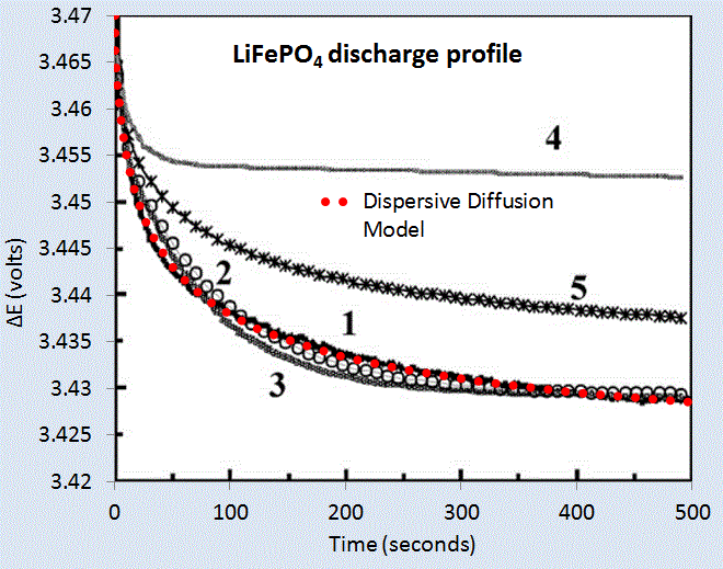Figure 5 : Discharge profile of LiFePO4 battery cell [1], with the red dotted line showing the parameterized dispersive diffusion model.  The curves labelled 1 through 5 show alternative models that the authors applied to fit the data. Only the dispersive diffusion model duplicates the fast drop-off and long-time scale decline.

Figure 6 below shows the fit to voltage characteristics of a LiSO4F cell, drawn as a red dotted line above the light gray data points. In this case the diffusional model by Delacourt shown in solid black is well outside acceptable agreement.

Figure 6 : Discharge profile of LiFeSO4F battery cell [2], with the red dotted line showing the parameterized dispersive diffusion model.  The black curve shows the model that the authors applied to fit the data. 

The question is why does this simple formulation work so well? As with many similar cases of characterizing disordered material, the fundamentally derived solution needs to be adjusted to take into account the uncertainty in the parameter space.  However, this step is not routinely performed and by adding modeling details (see [4]) to try to make up for a poor fit works only as a cosmetic heuristic.   In contrast, by performing the uncertainty quantification, like we did with the diffusion coefficient, the first-order solution works surprisingly well with no need for additional detail.

Constant Current Discharge
Instead of assuming that the particle size is L, we can say that the L is an average and apply the same maximum entropy spread in values.
$$  \large C(t) = \int_{0}^{\infty} C(t,x) \frac{1}{L} e^{-x/L} dx $$
this integrates straightforwardly to this concise representation:
$$ \large C(t) = C_0 \frac{1}{ L + {\sqrt{D_0 t}} } $$
The reason we do this is to allow us to recursively define the change in charge to a current. In  this case, to get current we need to differentiate the charge with respect to time.
$$ \large I(t) = \frac{dC(t)}{dt}  $$
This differentiates to the following expression
$$ \large I(t) = - \frac{C_0}{ (L + {\sqrt{D_0 t}})^2} \frac{1}{2 \sqrt{t}} $$
But note that we can insert C(t) back in to the expression
$$ \large I(t) = \frac{C(t)}{(L + {\sqrt{D_0 t}}) 2 \sqrt{t}} $$
Finally, since I(t) is a constant and we can set that to a value of I_constant. Then the charge has the following profile
$$ C(t) = C(0) - k_c I_{constant} (L + \sqrt{Dt}) 2 \sqrt{t} $$
or as a voltage decline
$$ V(t) = V(0) - k_v I_{constant} (L + \sqrt{Dt}) 2 \sqrt{t} $$
For a set of constant current values, we can compare this formulation against experimental data for LiFePO4 (shown as gray open circles) shown in Figure 7 below. A slight constant current offset (which may arise from unspecified shunting and/or series elements) was required to allow for the curves to align proportionally.  Even with that, it is clear that the dispersive diffusion formulation works better than the conventional model (solid black lines) except where the discharge is nearing completion.

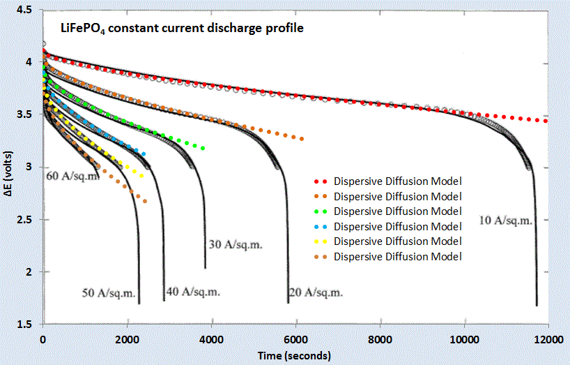Figure 7 : Constant current discharge profile [6]. Superimposed as dotted lines are the set of model fits which use the current value as a fixed parameter.

We can also model battery charging but the lack of information on the charging profile makes the discharge behavior a simpler study.

Related Diffusion Topics

• Dispersive Transport
• Corrosive Growth
• Dispersive Flow in Fractured Wells
• Diffusive CO2 Sequestration
• Ocean Heat Content

References

[1]

A. Churikov, A. Ivanishchev, I. Ivanishcheva, V. Sycheva, N. Khasanova, and E. Antipov, “Determination of lithium diffusion coefficient in LiFePO< sub> 4 electrode by galvanostatic and potentiostatic intermittent titration techniques,” Electrochimica Acta, vol. 55, no. 8, pp. 2939–2950, 2010.

[2]

C. Delacourt, M. Ati, and J. Tarascon, “Measurement of Lithium Diffusion Coefficient in Li y FeSO4F,” Journal of The Electrochemical Society, vol. 158, no. 6, pp. A741–A749, 2011.

[3]

M. Park, X. Zhang, M. Chung, G. B. Less, and A. M. Sastry, “A review of conduction phenomena in Li-ion batteries,” Journal of Power Sources, vol. 195, no. 24, pp. 7904–7929, Dec. 2010.

[4]

J. Christensen and J. Newman, “A mathematical model for the lithium-ion negative electrode solid electrolyte interphase,” Journal of The Electrochemical Society, vol. 151, no. 11, pp. A1977–A1988, 2004.

[5]

Q. Wang, H. Li, X. Huang, and L. Chen, “Determination of chemical diffusion coefficient of lithium ion in graphitized mesocarbon microbeads with potential relaxation technique,” Journal of The Electrochemical Society, vol. 148, no. 7, pp. A737–A741, 2001.

[6]

P. M. Gomadam, J. W. Weidner, R. A. Dougal, and R. E. White, “Mathematical modeling of lithium-ion and nickel battery systems,” Journal of Power Sources, vol. 110, no. 2, pp. 267–284, 2002.

[7]

“Hybrid and Electric Vehicle Engineering Academy.” [Online]. Available: http://training.sae.org/academies/acad06/. [Accessed: 09-Jun-2013].

The homework problem to end all homework problems

This is a problem that has driven anyone that has studied climate science up the wall.

Premise: Venus has an adiabatic index γ (gamma) and a temperature lapse rate λ (lambda). Earth also has an adiabatic index and temperature lapse rate.  These have been measured, and for the Earth a standard atmospheric profile has been established. The general relationship is based on thermodynamic principles but the shape of the profile diverges from simple applications of adiabatic principles.  In other words, a heuristic is applied to allow it to match the empirical observations, both for Venus and Earth. See this link for more background. 

Assigned Problem: Derive the adiabatic index and lapse rate for both planets, Venus and Earth, using only the planetary gravitational constant, the molar composition of atmospheric constituents, and any laws of physics that you can apply.  The answer has to be right on the mark with respect to the empirically-established standards.

Caveat: Reminder that this is a tough nut to crack.

Solution:  The approach to use is concise but somewhat twisty.  We work along two paths, the initial path uses basic physics and equations of continuity;  while the subsequent path ties the loose ends together using thermodynamic relationships which result in the familiar barometric formula and lapse rate formula.  The initial assumption that we make is to start with a sphere that forms a continuum from the origin; this forms the basis of a polytrope, a useful abstraction to infer the generic properties of planetary objects.

An abstracted planetary atmosphere

The atmosphere has a density ρ, that decreases outward from the origin. The basic laws we work with are the following:

Mass Conservation

$$ \frac{dm(r)}{dr} = 4 \pi r^2 \rho $$

Hydrostatic Equilibrium

$$ \frac{dP(r)}{dr} = - \rho g = - \frac{Gm(r)}{r^2}\rho $$

To convert to purely thermodynamic terms, we first integrate the hydrostatic equilibrium relationship over the volume of the sphere
$$ \int_0^R \frac{dP(r)}{dr} 4 \pi r^3 dr = 4 \pi R^3 P(R) - \int_0^R 12 P(r) \pi r^2 dr $$
on the right side we have integrated by parts, and eliminate the first term as P(R) goes to zero (note: upon review, the zeroing of P(R) is an approximation if we do not let R extend to the deep pressure vacuum of space, as we recover the differential form later -- right now we just assume P(R) decreases much faster than R^3 increases ). We then reduce the second term using the mass conservation relationship, while recovering the gravitational part:
$$ - 3 \int_0^M\frac{P}{\rho}dm = -\int_0^R 4 \pi r^3 \frac{G m(r)}{r^2} dr $$
again we apply the mass conservation
$$ - 3 \int_0^M\frac{P}{\rho}dm = -\int_0^M  \frac{G m(r)}{r} dm $$
The  right hand side is simply the total gravitational potential energy Ω while the left side reduces to a pressure to volume relationship:
 $$ - 3 \int_0^V P dV = \Omega$$
This becomes a variation of the Virial Theorem relating internal energy to potential energy.

Now we bring in the thermodynamic relationships, starting with the ideal gas law with its three independent variables. 

Ideal Gas Law

$$ PV = nRT $$

Gibbs Free Energy

$$ E = U - TS + PV $$

Specific Heat (in terms of molecular degrees of freedom)

$$ c_p = c_v + R = (N/2 + 1) R $$


On this path, we make the assertion that the Gibbs free energy will be minimized with respect to perturbations. i.e. a variational approach.

$$ dE = 0 = dU - d(TS) + d(PV) = dU - TdS - SdT + PdV + VdP $$

Noting that the system is closed with respect to entropy changes (an adiabatic or isentropic process) and substituting the ideal gas law featuring a molar gas constant for the last term.

$$ 0 = dU - SdT + PdV + VdP = dU - SdT + PdV + R_n dT$$

At constant pressure (dP=0) the temperature terms reduce to the specific heat at constant pressure:

$$ - S dT + nR dT = (c_v +R_n) dT = c_p dT $$

Rewriting the equation

$$ 0 = dU + c_p dT + P dV $$

Now we can recover the differential virial relationship derived earlier:

$$ - 3 P dV = d \Omega $$

and replace the unknown PdV term

$$ 0 = dU + c_p dT - d \Omega / 3 $$

but dU is the same potential energy term as dΩ, so

$$ 0 = 2/3 d \Omega+ c_p dT $$

Linearizing the potential gravitational energy change with respect to radius

$$ 0 = \frac{2 m g}{3} dr + c_p dT $$

Rearranging this term we have derived the lapse formula

$$ \frac{dT}{dr} = - \frac{mg}{3/2 c_p} $$

Reducing this in terms of the ideal gas constant and molecular degrees of freedom N

$$ \frac{dT}{dr} = - \frac{mg}{3/2 (N/2+1) R_n} $$

We still need to derive the adiabatic index, by coupling the lapse rate formula back to the hydrostatic equilibrium formulation.

Recall that the perfect adiabatic relationship (the Poisson's equation result describing the potential temperature) does not adequately describe a standard atmosphere -- being 50% off in lapse rate --  and so we must use a more general polytropic process approach.

Combining the Mass Conservation with the Hydrostatic Equilibrium:

$$ \frac{1}{r^2} \frac{d}{dr} (\frac{r^2}{\rho} \frac{dP}{dr}) = -4 \pi G \rho $$

if we make the substitution
$$ \rho = \rho_c \theta^n $$
where n is the polytropic index.  In terms of pressure via the ideal gas law
$$ P = P_c \theta^{n+1} $$
if we scale r as the dimensionless ξ :

$$ \frac{1}{\xi^2} \frac{d}{d\xi} (\frac{\xi^2}{\rho} \frac{dP}{d\xi}) = - \theta^n $$

This formulation is known as the Lane-Emden equation and is notable for resolving to a polytropic term. A solution for n=5 is
$$ \theta = ({1 + \xi^2/3})^{-1/2} $$

We now have a link to the polytropic process equation
$$ P V^\gamma = {constant} $$
and
$$ P^{1-\gamma} T^{\gamma} = {constant} $$
or
$$ P = P_0 (\frac{T}{T_0})^{\frac{\gamma}{1-\gamma}} $$
Tieing together the loose ends, we take our lapse rate gradient
$$ \frac{dT}{dr} = \frac{mg}{3/2 (N/2+1) R} $$
and convert that into an altitude profile, where r = z
$$ T = T_0 (1 - \frac{z}{f z_0}) $$
where
$$ z_0 = \frac{R T_0}{m g} $$
and
$$ f = 3/2 (1 + N/2) $$
and the temperature gradient, aka lapse rate
$$ \lambda=   \frac{m g}{ 3/2 (1 + N/2) R } $$
To generate a polytropic process equation from this, we merely have to raise the lapse rate to a power, so that we recreate the power law version of the barometric formula:
$$  P = P_0 (1 - \frac{z}{f z_0})^f $$
which essentially reduces to Poisson's equation on substitution:
$$ P = P_0 (T/T_0)^f $$
where the equivalent adiabatic exponent is
$$ f =  \frac{\gamma}{1-\gamma} $$

Now we have both the lapse rate, barometric formula, and Poisson's equation derived based only on the gravitational constant g, the gas law constant R, the average molar molecular weight of the atmospheric constituents m, and the average degrees of freedom N.

Answer: Now we want to check the results against the observed values for the two planets

Parameters

Object	Main Gas	N	m	g
Earth	N2, O2	5	28.96	9.807
Venus	CO2	6	43.44	8.87

Results

Object	Lapse Rate	observed	f	observed
Earth	6.506 C/km	6.5	21/4	5.25
Venus	7.72	7.72	6	6

All the numbers are spot on with respect to the empirical data recorded for both Earth and Venus, with supporting figures available here.

-------

The rough derivation that I previously posted to explain the empirical data was not very satisfying in its thoroughness.  The more comprehensive derivation in this post serves to shore up the mystery behind the deviation from the adiabatic derivation.  The key seems to be correctly accounting for the internal energy necessary to maintain the gravitational hydrostatic equilibrium. Since the polytropic expansion describes a process, the actual atmosphere can accommodate these constraints (while minimizing Gibbs free energy under constant entropy conditions) by selecting the appropriate polytropic index.   The mystery of the profile seems not so mysterious anymore.

Criticisms welcome as I have not run across anything like this derivation to explain the Earth's standard atmosphere profile nor the stable Venus data (not to mention the less stable Martian atmosphere).  The other big outer planets filled with hydrogen are still an issue, as they seem to follow the conventional adiabatic profile, according to the few charts I have access to.  The moon of Saturn, Titan, is an exception as it has a nitrogen atmosphere with methane as a greenhouse gas.

BTW, this post is definitely not dedicated to Ferenc Miskolczi. Please shoot me if I ever drift in that direction. It's a tough slog laying everything out methodically but worthwhile in the long run.

                      Added                     

Added Fig 1 : Lapse Rate on Earth versus Latitude. From

D. J. Lorenz and E. T. DeWeaver, “Tropopause height and zonal wind response to global warming in the IPCC scenario integrations,” Journal of Geophysical Research: Atmospheres (1984–2012), vol. 112, no. D10, 2007.

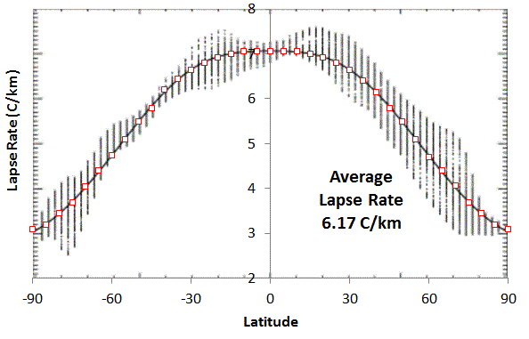Added Fig 2 : Lapse Rate on Earth versus Latitude. The average was calculated by integrating
with effective cross-sectional area weighting of (sin(Latitude+2.5)-sin(Latitude-2.5)) . Adapted from

J. P. Syvitski, S. D. Peckham, R. Hilberman, and T. Mulder, “Predicting the terrestrial flux of sediment to the global ocean: a planetary perspective,” Sedimentary Geology, vol. 162, no. 1, pp. 5–24, 2003.

Added Fig 3: This study also suggests an average lapse rate of 6.1C/km over the northern hemisphere.

I. Mokhov and M. Akperov, “Tropospheric lapse rate and its relation to surface temperature from reanalysis data,” Izvestiya, Atmospheric and Oceanic Physics, vol. 42, no. 4, pp. 430–438, 2006.

Since I posted this derivation, I received feedback from several other blogs which I attached as comments below this post.  In the original post I concluded by saying that I was satisfied with my alternate derivation, but after receiving the feedback, there is still the nagging issue of why the Venus lapse rate profile can be so linear in the lower atmosphere even though we know that the heat capacity of CO2 varies with temperature (particularly in the high temperature range of greater than 500 Kelvin).

If  we go back and look at the hydrostatic relation derived earlier, we see an interesting identity:
$$ - 3 \int_0^M\frac{P}{\rho}dm = -\int_0^M  \frac{G M}{r} dm $$
If I pull out the differential from the integral
$$ 3 \frac{P}{\rho} = \frac{G M}{r} $$
and then realize that the left-hand side is just the Ideal Gas law
$$ 3RT/m = \frac{G M}{r} $$
This is internal energy due to  gravitational potential energy.
If we take the derivative with respect to r, or altitude:
$$ 3R \frac{dT}{dr} = - \frac{G M m}{r^2} $$
The right side is just the gravitational force on an average particle. So we essentially can derive a lapse rate directly:
$$  \frac{dT}{dr} = - \frac{g m}{3 R} $$
This will generate a linear lapse rate profile of temperature that decreases with increasing altitude. Note however that this does not depend on the specific heat of the constituent atmospheric molecules. That is not surprising since it only uses the Ideal Gas law, with no application of the variational Gibbs Free Energy approach used earlier.

What this gives us is a universal lapse rate that does not depend on the specific heat capacity of the constituent gases, only the mean molar molecular weight, m.   This is of course an interesting turn of events in that it could explain the highly linear lapse  profile of Venus.  However, plugging in numbers for the gravity of Venus and the mean molecular weight (CO2 plus trace gases), we get a lapse rate that is precisely twice that which is observed.

The "obvious"  temptation is to suggest that half of the value of this derived hydrodynamic lapse rate would position it as the mean of the lapse rate gradient and an isothermal lapse rate (i.e. slope of zero).
$$  \frac{dT}{dr} = - \frac{g m}{6 R} $$
The rationale for this is that most of the planetary atmospheres are not any kind of equilibrium with energy flow and are constantly swinging between an insolating phase during daylight hours, and then a outward radiating phase at night.   The uncertainty is essentially describing fluctuations between when an atmosphere is isothermal (little change of temperature with altitude producing a MaxEnt outcome in distribution of pressures, leading to the classic barometric formula) or isentropic (where no heat is exchanged with the surroundings, but the temperature can vary as rapid convection occurs).

In keeping with the Bayesian decision making, the uncertainty is reflected by equal an weighting between isothermal (zero lapse rate gradient) and an isentropic (adiabatic derivation shown).  This puts the mean lapse rate at half the isentropic value. For Earth, the value of g*m/3R is 11.4 C/km.  Half of this value is 5.7 C/km, which is a value closer to actual mean value than the US Standard Atmosphere of 6.5 C/km

J. Levine, The Photochemistry of Atmospheres. Elsevier Science, 1985.
"The value chosen for the convective adjustment also influences the calculated surface temperature. In lower latitudes, the actual temperature decrease with height approximates the moist adiabatic rate. Convection transports H2O to higher elevations where condensation occurs, releasing latent heat to the atmosphere; this lapse rate, although variable, has an average annual value of 5.7 K/km in the troposphere. In mid and high latitudes, the actual lapse rates are more stable; the vertical temperature profile is controlled by eddies that are driven by horizontal temperature gradients and by topography. These so-called baroclinic processes produce an average lapse rate of 5.2 K/km - It is interesting to note that most radiative convective models have used a lapse rate of 6.5 K km - which was based on date sets extending back to 1933. We know now that a better hemispherical annual lapse rate is closer to 5.2 K/km, although there may be significant seasonal variations. "

BTW, the following references are very interesting presentations on the polytropic approach.


References

[1]

“Polytropes.” [Online]. Available: http://mintaka.sdsu.edu/GF/explain/thermal/polytropes.html. [Accessed: 19-May-2013].

[2]

B. Davies, “Stars Lecture.” [Online]. Available: http://www.ast.cam.ac.uk/~bdavies/Stars2 . [Accessed: 28-May-2013].

                      Even More Recent Research                    

A number of Chinese academics [3,4] are attacking the polytropic atmosphere problem from an angle that I hinted at in the original Standard Atmosphere Model and Uncertainty in Entropy post.    The gist of their approach is to assume that the atmosphere is not under thermodynamic equilibrium (which it isn't as it continuously exchanges heat with the sun and outer space in a stationary steady-state) and therefore use some ideas of non-extensible thermodynamics.  Specifically they invoke Tsallis entropy and a generalized Maxwell-Boltzmann distribution to model the behavioral move toward an equilibrium.  This is all in the context of self-gravitational systems, which is the theme of this post.  Why I think it is intriguing, is that they seem to tie the entropy considerations together with the polytropic process and arrive at some very simple relations (at least they appear somewhat simple to me).

In the non-extensive entropy approach, the original Maxwell-Boltzmann (MB) exponential velocity distribution is replaced with the Tsallis-derived generalized distribution -- which looks like the following power-law equation:

$$ f_q(v)=n_q B_q (\frac{m}{2 \pi k T})^{3/2} (1-(1-q) \frac{m v^2}{2 k T})^{\frac{1}{1-q}}$$

The so-called q-factor is a non-extensivity parameter which indicates how much the distribution deviates from MB statistics. As q approaches 1, the expression gradually trasforms into the familiar MB exponentially damped v^2 profile.

When q is slightly less than 1, all the thermodynamic gas equations change slightly in character.  In particular, the scientist Du postulated that the lapse rate follows the familiar linear profile, but scaled by the (1-q) factor:

$$ \frac{dT}{dr} = \frac{(1-q)g m}{R} $$

Note that this again has no dependence on the specific heat of the constituent gases, and only assumes an average molecular weight.  If q=7/6 or Q = 1-q = -1/6, we can model the f=6 lapse rate curve that we fit to earlier.

There is nothing special about the value of f=6 other than the claim that this polytropic exponent is on the borderline for maintaining a self-gravitational system [5].

Note that as q approaches unity, the thermodynamic equilibrium value, the lapse rate goes to zero, which is of course the maximum entropy condition of uniform temperature.

The Tsallis entropy approach is suspiciously close to solving the problem of the polytropic standard atmosphere. Read Zheng's paper for their take [3] and also Plastino [6]. 

The cut-off in the polytropic distribution (5) is an example of what is known, within the field of non extensive thermostatistics, as “Tsallis cut-off prescription”, which affects the q-maximum entropy distributions when q < 1. In the case of stellar polytropic distributions this cut-off arises naturally, and has a clear physical meaning. The cut-off corresponds, for each value of the radial coordinate r, to the corresponding gravitational escape velocity.

This has implications for the derivation of the homework problem that we solved at the top of this post, where we eliminated one term of the integration-by-parts solution. Obviously, the generalized MB formulation does have a limit to the velocity of a gas particle in comparison to the classical MB view. The tail in the statistics is actually cut-off as velocities greater than a certain value are not allowed, depending on the value of q.  As q approaches unity, the velocities allowed (i.e. escape velocity) approach infinity.

As Plastino states [6]:

Polytropic distributions happen to exhibit the form of q-MaxEnt distributions, that is, they constitute distribution functions in the (x,v) space that maximize the entropic functional Sq under the natural constraints imposed by the conservation of mass and energy.

The enduring question is does this describe our atmosphere adequately enough? Zheng and company certainly open it up to another interpretation.

[3]

Y. Zheng, W. Luo, Q. Li, and J. Li, “The polytropic index and adiabatic limit: Another interpretation to the convection stability criterion,” EPL (Europhysics Letters), vol. 102, no. 1, p. 10007, 2013.

[4]

Z. Liu, L. Guo, and J. Du, “Nonextensivity and the q-distribution of a relativistic gas under an external electromagnetic field,” Chinese Science Bulletin, vol. 56, no. 34, pp. 3689–3692, Dec. 2011.

[5]

M. V. Medvedev and G. Rybicki, “The Structure of Self-gravitating Polytropic Systems with n around 5,” The Astrophysical Journal, vol. 555, no. 2, p. 863, 2001.

[6]

A. Plastino, “Sq entropy and selfgravitating systems,” europhysics news, vol. 36, no. 6, pp. 208–210, 2005.

--