Ocean thermal expansion
The ocean absorbs heat per area according to its heat capacity$$ \Delta E = C_p \cdot \Delta T \cdot {Depth}$$
The linear coefficient of thermal expansion is assumed constant over a temperature range. Multiplying this over a depth:
$$ \Delta Z = \epsilon \cdot \Delta T \cdot Depth $$
But now we can substitute the total energy gained from the first equation:
$$ \Delta Z = \epsilon \frac{\Delta E}{C_p} $$
Assume that the linear coefficient of thermal expansion is 0.000207 per °C, and specific heat capacity is 4,000,000 J/m^3/°C.
If an excess forcing of 0.6 W/m^2 occurs over one year (see the OHC model), then the increase in the level of the ocean is
0.000207 * 0.6*(365*24*60*60) / 4,000,000 = 0.98 mm
This is called the steric sea-level rise, and it is just one component of the sea-level rise over time (the others have to do with melting ice). From the figure below, one can see that the thermal rise is close to 1mm/year over the last decade.
 |
| The red line shows the thermal expansion from the ocean heating. Thermal rise is 1 mm/year over the 3 mm/year total sea-level rise. |
Atmosphere thermal expansion
The trick here is to infer the atmosphere expansion by looking at an equal pressure point as a function of altitude (a geopotential height isobar) and determine how much that point has increased over time. I was able to find one piece of data from The Weather Channel's senior meteorologist Stu Ostro.The geopotential height anomaly is shown below for the 500 mb (1/2 atmosphere)
 |
| Geopotential height anomaly @ 500 mb plotted alongside global temperature anomaly. |
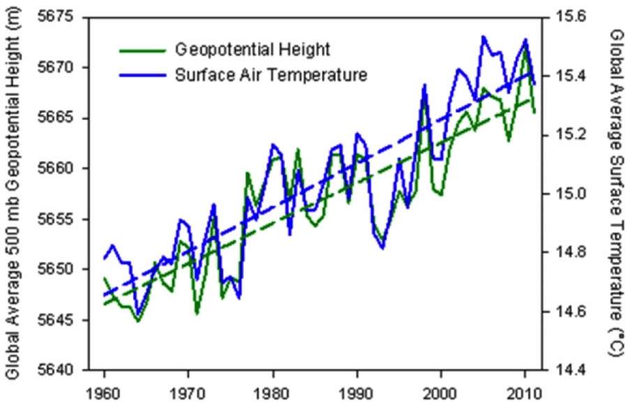 | |
| Global average geopotential height @ 500 mb plotted alongside global temperature. http://icons-ak.wxug.com/graphics/earthweek/geopotential-height-and-air-temperature.png |
To understand how the altitude has changed, consider the classical barometric formula:
$$ P(H) = P_0 e^{-mgH/RT} $$
We take the point at which we reached 1/2 the STP of 1 atmosphere at sea-level:
$$ P(H)/P_0 = 0.5 = e^{-mgH/RT} $$
or
$$ H = RT/mg \cdot ln(2) $$
Assuming the average molecular weight of the atmospheric gas constituents does not change, the change in altitude (H) should be related to the change in temperature (T) by:
$$ \Delta H = R \Delta T / mg \cdot ln(2) $$
or
$$ \frac{ \Delta H}{\Delta T} = \frac{R}{mg} ln(2) $$
For R = 8314, m=29, and g=9.8, the slope should be 29.25 *ln(2) = 20.3 m/°C.
From the linear regression agreement between the two, we get a value of 25.7 m/°C.
 |
| Linear regression between the geopotential height change and temperature change |
Why is this geopotential height change about 26% higher than it should be from the theoretical value considering that the height should track the temperature according to the barometric formula?
If we use the polytropic approximation (equation 1 in the barometric formula), the altitudinal difference between the low temperature and high temperature 500 mb pressure values remains the same as when we use the classic exponential damped barometric formula:
 |
| If we apply the polytropic barometric formula instead of the exponential, we still show a real height change that is higher than theoretically predicted by ~25% at the 500 mb isobar. |
This discrepancy could be due to measurement error, as the readings are taken by weather balloons and the accuracy could have drifted over the years.
It is also possible that the composition of the atmosphere could have changed slightly at altitude. What happens if the moisture increased slightly? This shouldn't make much difference.
Most likely is the possibility that the baseline sea-level pressure has changed, which shifted the 500 mbar point artificially. See http://www.ipcc.ch/publications_and_data/ar4/wg1/en/ch10s10-3-2-4.html.
"10.3.2.4 Sea Level Pressure and Atmospheric CirculationI will have to figure out the mean sea-level pressure change over this time period to verify this hypothesis.
As a basic component of the mean atmospheric circulations and weather patterns, projections of the mean sea level pressure for the medium scenario A1B are considered. Seasonal mean changes for DJF and JJA are shown in Figure 10.9 (matching results in Wang and Swail, 2006b). Sea level pressure differences show decreases at high latitudes in both seasons in both hemispheres. The compensating increases are predominantly over the mid-latitude and subtropical ocean regions, extending across South America, Australia and southern Asia in JJA, and the Mediterranean in DJF. Many of these increases are consistent across the models. This pattern of change, discussed further in Section 10.3.5.3, has been linked to an expansion of the Hadley Circulation and a poleward shift of the mid-latitude storm tracks (Yin, 2005). This helps explain, in part, the increases in precipitation at high latitudes and decreases in the subtropics and parts of the mid-latitudes. Further analysis of the regional details of these changes is given in Chapter 11. The pattern of pressure change implies increased westerly flows across the western parts of the continents. These contribute to increases in mean precipitation (Figure 10.9) and increased precipitation intensity (Meehl et al., 2005a). "
The following recent research article looks into the shifts in geopotential height over shorter time durations:
[1]
Y. Y. Hafez and M. Almazroui, “The Role Played by Blocking Systems over Europe in Abnormal Weather over Kingdom of Saudi Arabia in Summer 2010,” Advances in Meteorology, vol. 2013, p. 20, 2013.
ADDED 7/8/2013
One possibility for the larger-than-expected altitude change is that the average lapse rate has changed slightly. We can use the lapse rate variation of the barometric formula, and perturb the lapse rate, L, around its average value:
$$ P(H) = P(0) (1- \frac{LH}{T_0})^{\frac{gm}{LR}} $$
Granted, the error bars on this calculation are significant but we can see how subtle the effect is.
Sea-level pressure, P(0) = 1013.25 mb
Gas constant, R = 8.31446 J/K/mol
Earth's gravity, g = 9.807 m/s^2
Avg molecular weight, m = 0.02896 kg/m
In 1960, the temperature was about 14.65°C and 500 mb altitude was 5647 m.
In 2010, the temperature was about 15.4°C and 500 mb altitude was 5667 m.
All we need to do is invert the P(H) formula for each pair of values, modifying L slightly.
If we select a lapse rate, L, for 1960 of 0.0051°C/m, we calculate H = 5647.9m for P(H)=500 mb.
If we select a lapse rate, L, for 2010 of 0.0050°C/m, we calculate H = 5668.4m for P(H)=500 mb.
The difference in the two altitudes for a change in L of -0.0001°C/m is 20.5m, about what the geopotential height chart shows.
If we leave the L at 0.0051°C/m for both 1960 and 2010, the difference of the 500mb altitudes is only 14.7m.
To the extent that we can trust the numbers on the charts from Ostro, the change in geopotential height is suggesting a feedback effect in the lapse rate due to global warming. The lapse rate is decreasing over time, which implies that the heat capacity of the atmosphere is increasing (likely due to higher specific humidity), thereby buffering changes in temperature with altitude.
This means that a given temperature increase at a particular altitude (where the CO2 IR window can achieve a radiative balance) will be reflected as a scale-modified temperature at sea level
In 1960, the temperature difference at 500mb altitude is 0.0051°C/m * 5647.9m = 28.80°C
In 2010, the temperature difference at 500mb altitude is 0.0050°C/m * 5668.4m = 28.34°C
The difference at sea-level from the chart is 15.4°C-14.65°C = 0.75°C whereas the difference at the 500mb altitude assuming the modified lapse rate is 0.75°C - 0.46°C = 0.29°C. If the lapse rate didn't change then this sea-level difference would maintain at a constant atmospheric pressure isobar in altitude.
For implications in the interpretation, see page 24 of National Research Council Panel on Climate Change Feedbacks (2003). Understanding climate change feedbacks : National Academies Press. ISBN 978-0-309-09072-8. They caution that the measurements require some precision, otherwise the errors can multiply due to the differences between two large numbers.