Can we get behavioral information from something as seemingly random and chaotic as the Vostok ice core temperature data? Yes, as it turns out, performing a stochastic analysis of any time series can yield some very fundamental behaviors of the underlying process. The premise is that we can model the historical natural variability that occurs over hundreds of thousands of years by stochastic temperature movements.
I took the approach of modeling a bounded random walk from two different perspectives. In Part 1, I take the classic approach of applying the fundamental random walk hopping formulation.
Part 1 : Ornstein-Uhlenbeck Random Walk
Figure 1 below shows the Vostok data collected at roughly 20 to 600 year intervals and above that a simulated time series of a random walk process that has a similar variance.
 |
Fig. 1: Ornstein-Uhlenbeck Random Walk process (top green) emulates
Vostok temperature variations (below blue) |
The basic model I assume is that some type of random walk (red noise) statistics are a result of the earth’s climate inhabiting a very shallow energy well in its quiescent state. See the
Figure 2 below. The well is broad on the order of 10 degrees C, and relatively shallow. Within this potential well, the climate hovers in a metastable state whereby small positive feedbacks of CO
2, water vapor, or albedo can push it in either direction. The small amounts of perturbation needed to move the global temperature represents this shallowness.
 |
| Fig. 2 : Schematic of random walk behavior of a metastable system occupying a shallow quasi-equilibrium |
The model of correlated Markovian random walk, whereby the perturbation can go in either a positive or negative direction each year matches this shallow energy well model remarkably well. The random walk can't grow without bound as soft temperature constraints do exist, mainly from the negative feedback of the Stefan-Boltzmann law.
To model these soft constraints, what we do is put a proportional drag on the random walk so the walk produces a noticeable asymmetry on large excursions from the quiescent point, T
q (I don’t call it equilibrium because it is really a quasi-equilibrium). This generates a
reversion to the mean on the Markov random walk hopping direction, which is most commonly associated with the general
Ornstein-Uhlenbeck process.
The way that random walk works is that if something gets to a certain point proportionately to the square root of time, then you can often interpolate how far the excursion is in a fraction of this time, see
Figure 3 below.
$$ \Delta T = \sqrt{Dt} $$
 |
Fig. 3 : Multiscale Variance applied to Monte Carlo simulated random walk.
The classic Square Root random walk is shown for reference. |
|
The agreement with the Vostok data is illustrated by
Figure 4 below. The multiscale variance essentially takes all possible pairs of points and plots the square root of the average temperature as a function of the time interval,
L.
 |
| Fig. 4 : Multiscale variance of Vostok data |
The Ornstein-Uhlenbeck kernel solution has a simple formula for the variance:
$$Temperature(L) = F(L) = \sqrt{\frac{h}{2 \sigma}(1-e^{-2 \sigma L})}$$
where
h is the hop rate and
σ is the drag factor. We assume the mean is zero for convenience.
The very simple code for generating a Monte Carlo simulation and the multiscale variance is shown in the
awk code snippet below. The BEGIN portion sets up the random walk parameters and then performs a random flip to determine whether the temperature will move high or low. The movements labeled
A and
C in
Figure 2 correspond to random numbers less than 1/2 (positive hops) and the movements labeled
B and
D correspond to random numbers greater than 1/2 (negative hops). This nearly canonical form captures reversion to the mean well if the mean is set to zero.
The hopping rate,
h, corresponds to a diffusion coefficent of 0.0008 degrees^2/year and a drag parameter is set to 0.0012, where the drag causes a reversion to the mean for long times and the resulting hop rate is proportionally reduced according to how large the excursion is away from the mean.
BEGIN { ## Set up the Monte Carlo O-U model
N = 330000
hop = 0.02828
drag = 0.0012
T[0] = 0
srand()
for(i=1; i<N; i++) {
if(rand()<0.5) {
T[i] = T[i-1] + hop*(1-T[i-1]*drag)
} else {
T[i] = T[i-1] - hop*(1+T[i-1]*drag)
}
}
}
{} ## No stream input
END { ## Do the multiscale variance
L = N/2
while(L > 1) {
Sum = 0
for(i=1; i<=N/2; i++) {
Val = T[i] - T[i+int(L)]
Sum += Val * Val
}
print int(L) "\t" sqrt(Sum/(N/2))
L = 0.9*L
}
}
The END portion calculates the statistics for the time series
T(i). The multiscale variance is essentially described by the following correlation measure. All pairs are calculated for a variance and the result is normalized as a square root.
$$ F(L) = [\frac{2}{N}\sum_{j = 1}^{N/2} ( Y_j - Y_{j+L})^2]^{\frac{1}{2}} \quad \forall \quad L \lt N/2 $$
The O-U curve is shown in
Figure 4 by the red curve. The long time-scale fluctuations in the variance-saturated region are artifacts based on the relative shortness of the time series. If a longer time series is correlated then these fluctuations will damp out and match the O-U asymptote.
The results from 8 sequential Monte Carlo runs of several hundred thousand years are illustrated in
Figure 5 below. Note that on occasion the long term fluctuations coincide with the Vostok data. I am not suggesting that some external forcing factors aren’t triggering some of the movements, but it is interesting how much of the correlation structure shows up at the long time ranges just from random walk fluctuations.
 |
Fig. 5 : Multiscale Variance for Vostok data and
various sampled Ornstein-Uhlenbeck random walk processes |
In summary, the Vostok data illustrates the characteristic power-law correlation at shorter times and then it flattens out at longer times starting at about 10,000 years. This behavior results from the climate constraints of the maximum and minimum temperature bounds, set by the negative feedback of S-B at the high end and various factors at the low end. So to model the historical variations over a place like Vostok, we start with a random walk and modify it with an Ornstein-Uhlenbeck drag factor so that as the temperature starts walking closer to the rails, the random walk starts to slow down. By the same token, we give the diffusion coefficient a bit of a positive-feedback push when it starts to go away from the rail.
The question is whether the same random walk extends to the very short time periods ranging from years to a few centuries. Vostok doesn’t give this resolution as is seen from
Figure 4 but other data sets do. If we can somehow extend this set of data to a full temporal dynamic range, this would provide an fully stochastic model for local climatic variation.
Figure 6 below shows a Greenland core data set which provides better temporal resolution than the Vostok set.
http://www.ncdc.noaa.gov/paleo/metadata/noaa-icecore-2490.html
ftp://ftp.ncdc.noaa.gov/pub/data/paleo/icecore/greenland/summit/ngrip/ngrip2006d15n-ch4-t.txt
 |
| Fig. 6 : Full Greenland time series generated at one year intervals. |
Yet, this data is qualified by the caveat that the shorter time intervals are "reconstructed". You can see this by the smoother profile at a shorter time scale shown in
Figure 7.
 |
| Fig. 7 : At shorter scale note the spline averaging which smooths out the data. |
This smoothening reconstruction is a significant hurdle in extracting the actual random walk characteristics at short time scales. The green curve in
Figure 8 below illustrates the multiscale variance applied to the set of 50,000 data points. The upper blue curve is a Monte Carlo execution of the excursions assuming O-U diffusion at a resolution of 1 year, and the lower red curve is the multiscale variance applied after processing with a 250 point moving average filter.
 |
Fig. 8 : Multiscale Variance of Ornstein-Uhlenbeck process
does not match Greenland data (blue line)
unless a moving average filter of 250 points is applied (red line). |
Higher resolution temperature time series are available from various European cities. The strip chart
Figure 9 below shows a time series from Vienna starting from the 18th century.
 |
| Fig. 9 : Vienna Temperature time series |
The multiscale variance shown in
Figure 10 suggests that the data is uncorrelated and consists of white noise.
 |
Fig. 10 : Multiscale Variance on data shows flat variance due to uncorrelated white noise.
Rise at the end due to AGW at current duration. |
Sensitivity
This description in no way counters the GHG theory but is used to demonstrate how sensitive the earth’s climate is to small perturbations. The fact that the temperature in places such as Vostok follows this red noise O-U model so well, indicates that it should also be hypersensitive to artificial perturbations such as that caused by adding large amounts of relatively inert CO2 to the atmosphere. The good agreement with a Ornstein-Uhlenbeck process is proof that the climate is sensitive to perturbations, and the CO2 we have introduced is the added forcing function stimulus that the earth is responding to. For the moment it is going in the direction of the stimulus, and the red noise is along for the ride, unfortunately obscuring the observation at the short time scales we are operating under.
Figure 11 below shows a couple of shorter duration simulations using the Vostok parameters. Note that the natural fluctuations can occasionally obscure any warming that may occur. I explored this in the previous post where I calculated cumulative exceedance probabilities
here.
 |
| Fig. 11 : Simulated time series showing the scale of the red noise |
Extrapolating the Vostok data, for an arbitrary 100 year time span, a 0.75 degree or more temperature increase will occur with only a 3% probability. In other words the one we are in right now is a low chance occurrence. It is not implausible, but just that the odds are low.
Alternatively, one could estimate the fraction of the increase due to potential variability with some confidence interval attached to it. This will generate an estimate of uncertainty for the forced fraction versus the natural variability fraction.
The model of Ornstein-Uhlenbeck random walk could include a drift term to represent a forcing function. For a long term data series we keep this low so that it only reaches a maximum value after a specified point. In
Figure 12 below, a drift term of 0.0002 degrees/year causes an early variance increase after 5000 years. This may indeed have been a natural forcing function in the historical as it creates an inflection point that matches the data better than the non-forced Ornstein-Uhlenbeck process in
Figure 4.
 |
Fig. 12 : Adding a small biased positive forcing function to the hop rate creates a strong early variance
as the temperature shifts to warmer temperatures sooner |
 |
| Fig. 13 : Another simulation run which matches the early increase in variance seen in the data |
The code below illustrates the small bias parameter,
force, added to the diffusion term,
hop, which adds a small drift term that adds to the variance increase over a long time period.
BEGIN { ## Set up the Monte Carlo O-U model
N = 330000
hop = 0.02828
drag = 0.0012
force = 0.00015
T[0] = 0.0
srand()
for(i=1; i<N; i++) {
if(rand()<0.5) {
T[i] = T[i-1] + (hop+force)*(1-T[i-1]*drag)
} else {
T[i] = T[i-1] - (hop-force)*(1+T[i-1]*drag)
}
if(i%100 == 0) print T[i]
}
}
The final caveat is that these historical time series are all
localized data proxies or local temperature measurements. They likely give larger excursions than the globally averaged temperature. Alas, that data is hard to generate from paleoclimate data or human records.
Part 2 : Semi-Markov Model
The first part made the assumption that a random walk can generate the long-term temperature time series data. The random-walk generates a power-law of 1/2 in the multiscale variance and the Ornstein-Uhlenbeck master equation provides a reversion-to-the-mean mechanism. One has to look at the model results cross-eyed to see halfway good agreement, so that the validity of this approach for matching the data is ambiguous at best.
Because the temperature excursions don't have orders of magnitude in dynamic range, the power-law may be obscured by other factors. For example, the Vostok data shows large relative amounts of noise over the recent short duration intervals, while the Greenland appears heavily filtered.
That raises the question of whether an alternate stochastic mechanism is operational. If we consider the Greenland data as given, then we need a model that generates smooth and slow natural temperature variations at a short time scale, and not the erratic movements of Brownian motion that the O-U supplies.
One way to potentially proceed is to devise a
doubly stochastic model. Along the time dimension, the overall motions are longer term, with the hopping proceeding in one direction until the temperature reverses itself. This is very analogous to a semi-Markov model as described by D.R. Cox and often seen in phenomenon such as the
random telegraph signal as described in
The Oil ConunDRUM.
A semi-Markov process supplies a very disordered notion of periodicity to the physical behavior. It essentially occupies the space between a more-or-less periodic waveform, with the erratic motion of a pure random walk.
The math behind a semi-Markov process is very straightforward. On the temporal dimension, we apply a probability distribution for a run length,
t.
$$p(t) = \alpha e^{-\alpha t}$$
To calculate a variance of the temperature excursion,
T, we use the standard definition for the second moment.
$$\sigma_T\,^2 = \int_0^\infty T(t)^2 \cdot p(t) dt$$
Here,
p(t) is related to the autocorrelation describing long-range order and a typical PDF is a damped exponential:
$$p(t) = \alpha e^{- \alpha t}$$
The simplification we apply assumes that the short-term temperature excursion is
$$T(t) = \sqrt{D \cdot t}$$
Then to calculate a multiscale variance, we take the square root to convert it to the units of temperature,
$$ var(T) = \sqrt{\sigma_T\,^2}$$
we supply the parameterizations to the integration, and keep a running tally up to the multiscale time of interest,
L.
$$var(T(L)) = \sqrt{\int_0^L \alpha e^{-\alpha t} \, Dt \, dt} = \sqrt{D (1-e^{-\alpha L} (\alpha L+1))/\alpha}$$
That is all there is to it. We have a short concise formulation, which has exactly
two fitting parameters, one for shifting the time scale
$$ \tau = \frac{1}{\alpha}$$
and the diffusion parameter,
D, scaling the temperature excursion.
To test this model, we can do both an analytical fit and Monte Carlo simulation experiments.
We start with the Greenland data as that shows a wide dynamic range in temperature excursions, see
Figure 14 below.
 |
| Fig. 14 : Greenland multiscale variance with semi-Markov model |
The thought was that the Greenland temperature data was reconstructed, with the background white noise removed at the finest resolution. This model reveals the underlying movement of that temperature.
$$D = 0.25 \,\, \mathsf{degrees^2/year}$$
$$ \alpha = 0.005 \,\, \mathsf{year^{-1}}$$
A quick check for asymptotic variance is
$$ var_\infty = \sqrt{D/\alpha} = 7 ^\circ C $$
 |
| Fig. 15 : Simulation of Greenland data assuming Semi-Markov with first-order lag bounds. |
The simulation in
Figure 15 uses the code shown below. Instead of square root excursions, this uses first-order lag movements, which shows generally similar behavior as the analytical expression.
#include <math.h>
#include <stdio.h>
#include <stdlib.h>
#include <time.h>
main() { // Set up the Monte Carlo model
#define N 100000
double char_time = 100.0;
double hop = 0.02;
double drag = 0.03;
int flip = 1;
double *T = new double[2*N];
int n = 1;
int R, L, i;
double Sum, Val, rnd;
T[0] = 0.0;
srand ( time(NULL) );
while(n < N) {
flip = -flip;
rnd = (double)rand()/(double)RAND_MAX;
R = -(int)(char_time * log(rnd));
for(i=n; i<=n+R; i++)
if(flip<0) {
T[i] = T[i-1] + hop*(1-T[i-1]*drag);
} else {
T[i] = T[i-1] - hop*(1+T[i-1]*drag);
}
n += R;
}
// Do the multiscale variance
L = N/2;
while(L > 1) {
Sum = 0.0;
for(i=1; i<N/2; i++) {
Val = T[i] - T[i+L];
Sum += Val * Val;
}
printf("%i\t%g\n", L, sqrt(Sum/(N/2)));
L = 0.1*L;
}
}
Greenland shows large temperature volatility when compared against the ice core proxy measurements of the Antarctic. The semi-Markov model when applied to Vostok works well in explaining the data (see Figure 16), with the caveat that a uniform level of white noise is added to the variance profile. The white noise data is uncorrelated so adds the same background level independent of the time scale, i.e. it shows a flat variance. Whether this is due to instrumental uncertainty or natural variation, we can't tell.
 |
| Fig. 16 : Semi-Markov model applied to Vostok data |
Assuming a white noise level of 0.9 degrees, the parametric data is:
$$D = 0.25 \,\, \mathsf{degrees^2/century}$$
$$ \alpha = 0.018 \,\, \mathsf{century^{-1}}$$
The check for asymptotic variance is
$$ var_\infty = \sqrt{D/\alpha} = 3.7 ^\circ C $$
The remarkable result is that the Vostok temperature shows similar model agreement to Greenland but the semi-Markov changes are on the order of 100's of
centuries, instead of 100's of
years for Greenland.
Another Antarctic proxy location is EPICA, which generally agrees with Vostok but has a longer temperature record.
Figure 17 and
Figure 18 also demonstrates the effect of small sample simulations and how that smooths out with over-sampling.
 |
| Fig. 17 : EPICA data with model and simulation |
 |
| Fig. 18 : EPICA data with model and oversampling simulation |
Part 3 : Epilog
The semi-Markov model described in
Part 2 shows better agreement than the model of random walk with Ornstein-Uhlenbeck process described in
Part 1. This better agreement is explained by the likely longer-term order implicit in natural climate change. In other words, the herky-jerky movements of random walk are less well-suited as a process model than longer term stochastic reversing trends appear. The random walk character still exists but likely has a strong bias depending on whether the historical is warming or cooling.
If we can get more of these proxy records for other locations around the world, we should be able to produce better models for natural temperature variability, and thus estimate exceedance probabilities for temperature excursions within well-defined time scales. With that we can estimate whether current temperature trends are out of the ordinary in comparison to historical records.
I found more recent data for Greenland which indicates a likely shift in climate fluctuations starting approximately 10,000 years ago.
 |
| Fig. 19 : From http://www.gps.caltech.edu/~jess/ "The figure below shows the record of oxygen isotope variation, a proxy for air temperature, at the Greenland Summit over the past 110,000 years. The last 10,000 years, the Holocene, is marked by relative climatic stability when compared to the preceding glacial period where there are large and very fast transitions between cold and warm times." | |
The data in
Figure 19 above and
Figure 20 below should be compared to the Greenland data described earlier, which ranged from 30,000 to 80,000 years ago.
 |
Fig. 20 : Multiscale variance of Greenland data over the last 10,000 years, not converted to temperature.
Note the flat white noise until several thousand years ago, when a noticeable uptick starts. |
The recent data definitely shows a more stable warmer regime than the erratic downward fluctuations of the past interglacial years. So the distinction is one between recent times and those of older than approximately 5,000 years ago.
See the post and comments on Climate Etc. regarding
climate sensitivity. The following chart (
Figure 21) illustrates possible mechanisms for a climate well. Notice the potential for an asymmetry in the potential barriers on the cool versus warm side.
 |
| Fig. 21: First Order Climate Well |
The following
Figure 22 is processed from the 30,000 to 80,000 year range Greenland ice core data. The histogram of cooling and warming rates is tabulated across the extremes (a) on the cool side below average (b) and on the warm side above average (c). Note the fast regime for warming on the warm side.
 |
Fig. 22 : Detection of Skewed Well.
On the high side of paleo temperatures, a fast temperature rate change is observed.
A range of these these rates is equally likely, indicating a fast transition between warm and extreme. |
Compare that to
Figure 23 over the last 10,000 years (the Holocene era) in Greenland. The split is that rates appear to accelerate as a region transitions from cold to warm and then vice versa. I think we can't make too much out of this effect as the recent Holocene-era data in Greenland is very noisy and often appears to jump between extremes in temperature in consecutive data points. As described earlier this is characteristic of white noise (and perhaps even aliasing) since no long-range order is observed. More recent high resolution research
has been published [1] but the raw data is not yet available. The claim is that the climate in Greenland during the Holocene appears highly sensitive to variations in environmental factors, which I find not too surprising.
 |
Fig. 23 : Greenland last 10,000 years.
Note the slope emphasis on the warm side versus the cold side of temperature regime. |
[1] Kobashi, T., K. Kawamura, J. P. Severinghaus, J.‐M. Barnola, T. Nakaegawa, B. M. Vinther, S. J. Johnsen, and J. E. Box (2011),
High variability of Greenland surface temperature over the past 4000 years estimated from trapped air in an ice core, Geophys. Res. Lett., 38, L21501, doi:10.1029/2011GL049444.
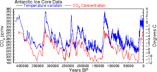
The following two figures show an interesting view of the random walk character of the Vostok CO2 and temperature data. A linear, non-sigmoid, shape indicates that the sampled data is occupying a uniform space between the endpoints. The raw CO2 shows this linearity (
Figure 24) while only the log of the temperature has the same linearity (
Figure 25). They both have similar correlation coefficients so that it is almost safe to assume that the two statistically track one another with this relation:
$$ ln(T-T_0) = k [CO2] + constant$$
or
$$ T = T_0 + c e^{k [CO2]}$$
This is odd because it is the opposite of the generally agreed upon dependence of the GHG forcing, whereby the log of the atmospheric CO2 concentration generates a linear temperature increase.
 |
| Fig.24: Rank histogram of CO2 excursions shows extreme linearity over range, indicating an ergodic mapping of a doubly stochastic random walk. The curl at the endpoints indicate the Ornstein-Uhlenbeck endpoints. |
 |
Fig. 25: Rank histogram of log temperature excursions shows extreme linearity over range.
The curl at the endpoints indicate the Ornstein-Uhlenbeck endpoints. |
 |
Fig. 26: Regular histogram for CO2. Regression line is flat but uniformity
is not as apparent because of noise due to the binning size. |


