This is a continuation from the Thermal Diffusion and Missing Heat post.
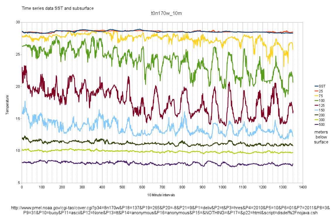
If one takes several months worth of data from a location, the sea surface temperature (SST) and subsurface time series looks like this over a few days.
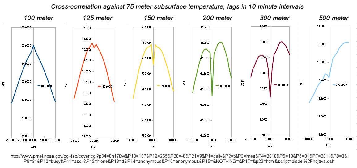
After a cross-correlation function is applied 75 meters downward, one sees an obvious yet small lag from that level as it mixes with the lower layers.
The lag is longer the farther the reach extends downward. If one assumes a typical James Hansen diffusion coefficient of 1.5 cm^2/s, the diffusion is actually very slow over long distance. A Fickian diffusion would only displace 100 meters after 3 years at that rate. So the effect is fairly subtle and to detect it requires some sophisticated data processing.
Bottom-line is that the surface water is heated and it does mix with the deeper waters. Otherwise, one would not see the obvious thermal mixing as is obtained from the TAO sites.
Some other correlations using R. These show longer range correlations. Note the strong correlation oscillations which indicates that temperatures changes happen in unison and in a coherent fashion, given a lag that is less apparent at this scale. Note that the lag is in the opposite direction due to the specification that R uses for defining an ACF ( x(t+k)*y(t), instead of x(t)*y(t+k)).
Thermal mixing and an effective diffusivity is occurring. The only
premise required is that an energy imbalance is occurring and that it
will continue to occur as CO2 is above the historical atmospheric
average. This imbalance shows up to a large extent in the oceans waters
and is reflected as a temporal lag in global warming.
Notes:
Have to be careful about missing data in certain sites. Any time you see a discontinuity in a correlation function, bad data (values with -9.999 typically) is usually responsible.


No comments:
Post a Comment