Wave Energy Spectrum

Ocean waves are just as disordered as the wind. We may not notice this because the scale of waves is usually smaller. In practice, the wind energy distribution relates to an open water wave energy distribution via similar maximum entropy disorder considerations. The following derivation assumes a deep enough water such that troughs do not touch bottom

First, we make a maximum entropy estimation of the energy of a one-dimensional propagating wave driven by a prevailing wind direction. The mean energy of the wave is related to the wave height by the square of the height, H. This makes sense because a taller wave needs a broader base to support that height, leading to a scaled pseudo-triangular shape, as shown in Figure 1 below.

Figure 1: Total energy in a directed wave goes as the square of the height, and the macroscopic fluid
properties suggest that it scales to size. This leads to a dispersive form for the wave size distribution

 Since the area of such a scaled triangle goes as H^2, the MaxEnt cumulative probability is:

$$ P(H) = e^{-a H^2} $$

where a is related to the mean energy of an ensemble of waves. This relationship is empirically observed from measurements of ocean wave heights over a sufficient time period. However, we can proceed further and try to derive the dispersion results of wave frequency, which is the very common oceanography measure. So we consider -- based on the energy stored in a specific wave -- the time, t, it will take to drop a height, H, by the Newton's law relation:

$$ t^2 \sim H $$

and since t goes as 1/f, then we can create a new PDF from the height cumulative as follows:

$$ p(f) df = \frac{dP(H)}{dH} \frac{dH}{df} df $$

where

$$ H \sim \frac{1}{f^2} $$

$$ \frac{dH}{df} \sim -\frac{1}{f^3} $$

then

$$ p(f) \sim \frac{1}{f^5} e^{-\frac{c}{f^4}} $$

which is just the Pierson-Moskowitz wave spectra that oceanographers have observed for years (developed first in 1964, variations of this include the Bretschneider and ITTC wave spectra) .

This concise derivation works well despite the correct path of calculating an auto-correlation from p(f) and then deriving a power spectrum from the Fourier Transform of p(f). Yet this convenient shortcut remains useful in understanding the simple physics and probabilities involved.



As we have an interest in using this derived form for an actual potential application, we can seek out public-access stations to obtain and evaluate some real data. The following Figure 2 is data pulled from the first region I accessed -- a pair of measuring stations located off the coast of San Diego. The default data selector picked the first day of this year, 1/1/2012 and the station server provided an averaged wave spectra for the entire day.  The red points correspond to best fits from the derived MaxEnt algorithm to the blue data set.

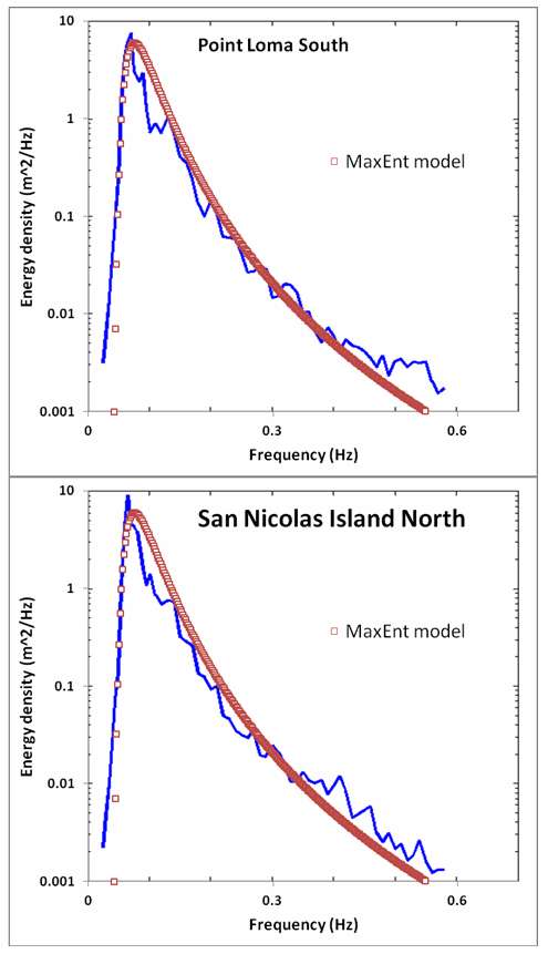Figure 2: Wave energy spectra from two sites off of the San Diego coastal region.
The Maximum Entropy estimate is in red.

To explore the dataset, here is a link to the interactive page :
http://cdip.ucsd.edu/?nav=historic&sub=data&units=metric&tz=UTC&pub=public&map_stati=1,2,3&stn=167&stream=p1&xyrmo=201201&xitem=product25

Like the wind energy spectrum, the wave spectrum derives simply from maximum entropy conditions.

Refs
Introduction to physical oceanography, RH Stewart