The homework problem to end all homework problems

This is a problem that has driven anyone that has studied climate science up the wall.

Premise: Venus has an adiabatic index γ (gamma) and a temperature lapse rate λ (lambda). Earth also has an adiabatic index and temperature lapse rate.  These have been measured, and for the Earth a standard atmospheric profile has been established. The general relationship is based on thermodynamic principles but the shape of the profile diverges from simple applications of adiabatic principles.  In other words, a heuristic is applied to allow it to match the empirical observations, both for Venus and Earth. See this link for more background. 

Assigned Problem: Derive the adiabatic index and lapse rate for both planets, Venus and Earth, using only the planetary gravitational constant, the molar composition of atmospheric constituents, and any laws of physics that you can apply.  The answer has to be right on the mark with respect to the empirically-established standards.

Caveat: Reminder that this is a tough nut to crack.

Solution:  The approach to use is concise but somewhat twisty.  We work along two paths, the initial path uses basic physics and equations of continuity;  while the subsequent path ties the loose ends together using thermodynamic relationships which result in the familiar barometric formula and lapse rate formula.  The initial assumption that we make is to start with a sphere that forms a continuum from the origin; this forms the basis of a polytrope, a useful abstraction to infer the generic properties of planetary objects.

An abstracted planetary atmosphere

The atmosphere has a density ρ, that decreases outward from the origin. The basic laws we work with are the following:

Mass Conservation

$$ \frac{dm(r)}{dr} = 4 \pi r^2 \rho $$

Hydrostatic Equilibrium

$$ \frac{dP(r)}{dr} = - \rho g = - \frac{Gm(r)}{r^2}\rho $$

To convert to purely thermodynamic terms, we first integrate the hydrostatic equilibrium relationship over the volume of the sphere
$$ \int_0^R \frac{dP(r)}{dr} 4 \pi r^3 dr = 4 \pi R^3 P(R) - \int_0^R 12 P(r) \pi r^2 dr $$
on the right side we have integrated by parts, and eliminate the first term as P(R) goes to zero (note: upon review, the zeroing of P(R) is an approximation if we do not let R extend to the deep pressure vacuum of space, as we recover the differential form later -- right now we just assume P(R) decreases much faster than R^3 increases ). We then reduce the second term using the mass conservation relationship, while recovering the gravitational part:
$$ - 3 \int_0^M\frac{P}{\rho}dm = -\int_0^R 4 \pi r^3 \frac{G m(r)}{r^2} dr $$
again we apply the mass conservation
$$ - 3 \int_0^M\frac{P}{\rho}dm = -\int_0^M  \frac{G m(r)}{r} dm $$
The  right hand side is simply the total gravitational potential energy Ω while the left side reduces to a pressure to volume relationship:
 $$ - 3 \int_0^V P dV = \Omega$$
This becomes a variation of the Virial Theorem relating internal energy to potential energy.

Now we bring in the thermodynamic relationships, starting with the ideal gas law with its three independent variables. 

Ideal Gas Law

$$ PV = nRT $$

Gibbs Free Energy

$$ E = U - TS + PV $$

Specific Heat (in terms of molecular degrees of freedom)

$$ c_p = c_v + R = (N/2 + 1) R $$


On this path, we make the assertion that the Gibbs free energy will be minimized with respect to perturbations. i.e. a variational approach.

$$ dE = 0 = dU - d(TS) + d(PV) = dU - TdS - SdT + PdV + VdP $$

Noting that the system is closed with respect to entropy changes (an adiabatic or isentropic process) and substituting the ideal gas law featuring a molar gas constant for the last term.

$$ 0 = dU - SdT + PdV + VdP = dU - SdT + PdV + R_n dT$$

At constant pressure (dP=0) the temperature terms reduce to the specific heat at constant pressure:

$$ - S dT + nR dT = (c_v +R_n) dT = c_p dT $$

Rewriting the equation

$$ 0 = dU + c_p dT + P dV $$

Now we can recover the differential virial relationship derived earlier:

$$ - 3 P dV = d \Omega $$

and replace the unknown PdV term

$$ 0 = dU + c_p dT - d \Omega / 3 $$

but dU is the same potential energy term as dΩ, so

$$ 0 = 2/3 d \Omega+ c_p dT $$

Linearizing the potential gravitational energy change with respect to radius

$$ 0 = \frac{2 m g}{3} dr + c_p dT $$

Rearranging this term we have derived the lapse formula

$$ \frac{dT}{dr} = - \frac{mg}{3/2 c_p} $$

Reducing this in terms of the ideal gas constant and molecular degrees of freedom N

$$ \frac{dT}{dr} = - \frac{mg}{3/2 (N/2+1) R_n} $$

We still need to derive the adiabatic index, by coupling the lapse rate formula back to the hydrostatic equilibrium formulation.

Recall that the perfect adiabatic relationship (the Poisson's equation result describing the potential temperature) does not adequately describe a standard atmosphere -- being 50% off in lapse rate --  and so we must use a more general polytropic process approach.

Combining the Mass Conservation with the Hydrostatic Equilibrium:

$$ \frac{1}{r^2} \frac{d}{dr} (\frac{r^2}{\rho} \frac{dP}{dr}) = -4 \pi G \rho $$

if we make the substitution
$$ \rho = \rho_c \theta^n $$
where n is the polytropic index.  In terms of pressure via the ideal gas law
$$ P = P_c \theta^{n+1} $$
if we scale r as the dimensionless ξ :

$$ \frac{1}{\xi^2} \frac{d}{d\xi} (\frac{\xi^2}{\rho} \frac{dP}{d\xi}) = - \theta^n $$

This formulation is known as the Lane-Emden equation and is notable for resolving to a polytropic term. A solution for n=5 is
$$ \theta = ({1 + \xi^2/3})^{-1/2} $$

We now have a link to the polytropic process equation
$$ P V^\gamma = {constant} $$
and
$$ P^{1-\gamma} T^{\gamma} = {constant} $$
or
$$ P = P_0 (\frac{T}{T_0})^{\frac{\gamma}{1-\gamma}} $$
Tieing together the loose ends, we take our lapse rate gradient
$$ \frac{dT}{dr} = \frac{mg}{3/2 (N/2+1) R} $$
and convert that into an altitude profile, where r = z
$$ T = T_0 (1 - \frac{z}{f z_0}) $$
where
$$ z_0 = \frac{R T_0}{m g} $$
and
$$ f = 3/2 (1 + N/2) $$
and the temperature gradient, aka lapse rate
$$ \lambda=   \frac{m g}{ 3/2 (1 + N/2) R } $$
To generate a polytropic process equation from this, we merely have to raise the lapse rate to a power, so that we recreate the power law version of the barometric formula:
$$  P = P_0 (1 - \frac{z}{f z_0})^f $$
which essentially reduces to Poisson's equation on substitution:
$$ P = P_0 (T/T_0)^f $$
where the equivalent adiabatic exponent is
$$ f =  \frac{\gamma}{1-\gamma} $$

Now we have both the lapse rate, barometric formula, and Poisson's equation derived based only on the gravitational constant g, the gas law constant R, the average molar molecular weight of the atmospheric constituents m, and the average degrees of freedom N.

Answer: Now we want to check the results against the observed values for the two planets

Parameters

Object	Main Gas	N	m	g
Earth	N2, O2	5	28.96	9.807
Venus	CO2	6	43.44	8.87

Results

Object	Lapse Rate	observed	f	observed
Earth	6.506 C/km	6.5	21/4	5.25
Venus	7.72	7.72	6	6

All the numbers are spot on with respect to the empirical data recorded for both Earth and Venus, with supporting figures available here.

-------

The rough derivation that I previously posted to explain the empirical data was not very satisfying in its thoroughness.  The more comprehensive derivation in this post serves to shore up the mystery behind the deviation from the adiabatic derivation.  The key seems to be correctly accounting for the internal energy necessary to maintain the gravitational hydrostatic equilibrium. Since the polytropic expansion describes a process, the actual atmosphere can accommodate these constraints (while minimizing Gibbs free energy under constant entropy conditions) by selecting the appropriate polytropic index.   The mystery of the profile seems not so mysterious anymore.

Criticisms welcome as I have not run across anything like this derivation to explain the Earth's standard atmosphere profile nor the stable Venus data (not to mention the less stable Martian atmosphere).  The other big outer planets filled with hydrogen are still an issue, as they seem to follow the conventional adiabatic profile, according to the few charts I have access to.  The moon of Saturn, Titan, is an exception as it has a nitrogen atmosphere with methane as a greenhouse gas.

BTW, this post is definitely not dedicated to Ferenc Miskolczi. Please shoot me if I ever drift in that direction. It's a tough slog laying everything out methodically but worthwhile in the long run.

                      Added                     

Added Fig 1 : Lapse Rate on Earth versus Latitude. From

D. J. Lorenz and E. T. DeWeaver, “Tropopause height and zonal wind response to global warming in the IPCC scenario integrations,” Journal of Geophysical Research: Atmospheres (1984–2012), vol. 112, no. D10, 2007.

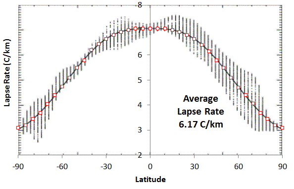
Added Fig 2 : Lapse Rate on Earth versus Latitude. The average was calculated by integrating
with effective cross-sectional area weighting of (sin(Latitude+2.5)-sin(Latitude-2.5)) . Adapted from

J. P. Syvitski, S. D. Peckham, R. Hilberman, and T. Mulder, “Predicting the terrestrial flux of sediment to the global ocean: a planetary perspective,” Sedimentary Geology, vol. 162, no. 1, pp. 5–24, 2003.

Added Fig 3: This study also suggests an average lapse rate of 6.1C/km over the northern hemisphere.

I. Mokhov and M. Akperov, “Tropospheric lapse rate and its relation to surface temperature from reanalysis data,” Izvestiya, Atmospheric and Oceanic Physics, vol. 42, no. 4, pp. 430–438, 2006.

Since I posted this derivation, I received feedback from several other blogs which I attached as comments below this post.  In the original post I concluded by saying that I was satisfied with my alternate derivation, but after receiving the feedback, there is still the nagging issue of why the Venus lapse rate profile can be so linear in the lower atmosphere even though we know that the heat capacity of CO2 varies with temperature (particularly in the high temperature range of greater than 500 Kelvin).

If  we go back and look at the hydrostatic relation derived earlier, we see an interesting identity:
$$ - 3 \int_0^M\frac{P}{\rho}dm = -\int_0^M  \frac{G M}{r} dm $$
If I pull out the differential from the integral
$$ 3 \frac{P}{\rho} = \frac{G M}{r} $$
and then realize that the left-hand side is just the Ideal Gas law
$$ 3RT/m = \frac{G M}{r} $$
This is internal energy due to  gravitational potential energy.
If we take the derivative with respect to r, or altitude:
$$ 3R \frac{dT}{dr} = - \frac{G M m}{r^2} $$
The right side is just the gravitational force on an average particle. So we essentially can derive a lapse rate directly:
$$  \frac{dT}{dr} = - \frac{g m}{3 R} $$
This will generate a linear lapse rate profile of temperature that decreases with increasing altitude. Note however that this does not depend on the specific heat of the constituent atmospheric molecules. That is not surprising since it only uses the Ideal Gas law, with no application of the variational Gibbs Free Energy approach used earlier.

What this gives us is a universal lapse rate that does not depend on the specific heat capacity of the constituent gases, only the mean molar molecular weight, m.   This is of course an interesting turn of events in that it could explain the highly linear lapse  profile of Venus.  However, plugging in numbers for the gravity of Venus and the mean molecular weight (CO2 plus trace gases), we get a lapse rate that is precisely twice that which is observed.

The "obvious"  temptation is to suggest that half of the value of this derived hydrodynamic lapse rate would position it as the mean of the lapse rate gradient and an isothermal lapse rate (i.e. slope of zero).
$$  \frac{dT}{dr} = - \frac{g m}{6 R} $$
The rationale for this is that most of the planetary atmospheres are not any kind of equilibrium with energy flow and are constantly swinging between an insolating phase during daylight hours, and then a outward radiating phase at night.   The uncertainty is essentially describing fluctuations between when an atmosphere is isothermal (little change of temperature with altitude producing a MaxEnt outcome in distribution of pressures, leading to the classic barometric formula) or isentropic (where no heat is exchanged with the surroundings, but the temperature can vary as rapid convection occurs).

In keeping with the Bayesian decision making, the uncertainty is reflected by equal an weighting between isothermal (zero lapse rate gradient) and an isentropic (adiabatic derivation shown).  This puts the mean lapse rate at half the isentropic value. For Earth, the value of g*m/3R is 11.4 C/km.  Half of this value is 5.7 C/km, which is a value closer to actual mean value than the US Standard Atmosphere of 6.5 C/km

J. Levine, The Photochemistry of Atmospheres. Elsevier Science, 1985.
"The value chosen for the convective adjustment also influences the calculated surface temperature. In lower latitudes, the actual temperature decrease with height approximates the moist adiabatic rate. Convection transports H2O to higher elevations where condensation occurs, releasing latent heat to the atmosphere; this lapse rate, although variable, has an average annual value of 5.7 K/km in the troposphere. In mid and high latitudes, the actual lapse rates are more stable; the vertical temperature profile is controlled by eddies that are driven by horizontal temperature gradients and by topography. These so-called baroclinic processes produce an average lapse rate of 5.2 K/km - It is interesting to note that most radiative convective models have used a lapse rate of 6.5 K km - which was based on date sets extending back to 1933. We know now that a better hemispherical annual lapse rate is closer to 5.2 K/km, although there may be significant seasonal variations. "

BTW, the following references are very interesting presentations on the polytropic approach.


References

[1]

“Polytropes.” [Online]. Available: http://mintaka.sdsu.edu/GF/explain/thermal/polytropes.html. [Accessed: 19-May-2013].

[2]

B. Davies, “Stars Lecture.” [Online]. Available: http://www.ast.cam.ac.uk/~bdavies/Stars2 . [Accessed: 28-May-2013].

                      Even More Recent Research                    

A number of Chinese academics [3,4] are attacking the polytropic atmosphere problem from an angle that I hinted at in the original Standard Atmosphere Model and Uncertainty in Entropy post.    The gist of their approach is to assume that the atmosphere is not under thermodynamic equilibrium (which it isn't as it continuously exchanges heat with the sun and outer space in a stationary steady-state) and therefore use some ideas of non-extensible thermodynamics.  Specifically they invoke Tsallis entropy and a generalized Maxwell-Boltzmann distribution to model the behavioral move toward an equilibrium.  This is all in the context of self-gravitational systems, which is the theme of this post.  Why I think it is intriguing, is that they seem to tie the entropy considerations together with the polytropic process and arrive at some very simple relations (at least they appear somewhat simple to me).

In the non-extensive entropy approach, the original Maxwell-Boltzmann (MB) exponential velocity distribution is replaced with the Tsallis-derived generalized distribution -- which looks like the following power-law equation:

$$ f_q(v)=n_q B_q (\frac{m}{2 \pi k T})^{3/2} (1-(1-q) \frac{m v^2}{2 k T})^{\frac{1}{1-q}}$$

The so-called q-factor is a non-extensivity parameter which indicates how much the distribution deviates from MB statistics. As q approaches 1, the expression gradually trasforms into the familiar MB exponentially damped v^2 profile.

When q is slightly less than 1, all the thermodynamic gas equations change slightly in character.  In particular, the scientist Du postulated that the lapse rate follows the familiar linear profile, but scaled by the (1-q) factor:

$$ \frac{dT}{dr} = \frac{(1-q)g m}{R} $$

Note that this again has no dependence on the specific heat of the constituent gases, and only assumes an average molecular weight.  If q=7/6 or Q = 1-q = -1/6, we can model the f=6 lapse rate curve that we fit to earlier.

There is nothing special about the value of f=6 other than the claim that this polytropic exponent is on the borderline for maintaining a self-gravitational system [5].

Note that as q approaches unity, the thermodynamic equilibrium value, the lapse rate goes to zero, which is of course the maximum entropy condition of uniform temperature.

The Tsallis entropy approach is suspiciously close to solving the problem of the polytropic standard atmosphere. Read Zheng's paper for their take [3] and also Plastino [6]. 

The cut-off in the polytropic distribution (5) is an example of what is known, within the field of non extensive thermostatistics, as “Tsallis cut-off prescription”, which affects the q-maximum entropy distributions when q < 1. In the case of stellar polytropic distributions this cut-off arises naturally, and has a clear physical meaning. The cut-off corresponds, for each value of the radial coordinate r, to the corresponding gravitational escape velocity.

This has implications for the derivation of the homework problem that we solved at the top of this post, where we eliminated one term of the integration-by-parts solution. Obviously, the generalized MB formulation does have a limit to the velocity of a gas particle in comparison to the classical MB view. The tail in the statistics is actually cut-off as velocities greater than a certain value are not allowed, depending on the value of q.  As q approaches unity, the velocities allowed (i.e. escape velocity) approach infinity.

As Plastino states [6]:

Polytropic distributions happen to exhibit the form of q-MaxEnt distributions, that is, they constitute distribution functions in the (x,v) space that maximize the entropic functional Sq under the natural constraints imposed by the conservation of mass and energy.

The enduring question is does this describe our atmosphere adequately enough? Zheng and company certainly open it up to another interpretation.

[3]

Y. Zheng, W. Luo, Q. Li, and J. Li, “The polytropic index and adiabatic limit: Another interpretation to the convection stability criterion,” EPL (Europhysics Letters), vol. 102, no. 1, p. 10007, 2013.

[4]

Z. Liu, L. Guo, and J. Du, “Nonextensivity and the q-distribution of a relativistic gas under an external electromagnetic field,” Chinese Science Bulletin, vol. 56, no. 34, pp. 3689–3692, Dec. 2011.

[5]

M. V. Medvedev and G. Rybicki, “The Structure of Self-gravitating Polytropic Systems with n around 5,” The Astrophysical Journal, vol. 555, no. 2, p. 863, 2001.

[6]

A. Plastino, “Sq entropy and selfgravitating systems,” europhysics news, vol. 36, no. 6, pp. 208–210, 2005.

--

Airborne fraction of CO2 explained by sequestering model

As acknowledgement of the atmospheric levels of CO2 reaching 400 PPM, this post is meant to clear up one important misconception (suggested prerequisite reading on fat-tail CO2 sequestration here and the significance of the fat-tail here)

A recently active skeptic meme is that the amount of CO2 as an airborne fraction is decreasing over time.

"If we look at the data since Mauna Loa started, we see that the percentage of the CO2 emitted by humans that “remains” in the atmosphere has averaged around half, but that it has diminished over time, by around 1% per decade.
Over the 30 year period 1959-1989 it was around 55%; over the following 20+ years it was just over 50%.
Why is this?"

What the befuddled fellow is talking about are the charts being shown below. These are being shown without much context and no supporting documentation, which puts the burden on the climate scientists to explain. Note that the airborne fraction does seem to decrease slightly over the past 50 years, even though the carbon emissions are increasing.

This obviously needs some explaining.  The following figure illustrates what the CO2 sequestration model actually does.

Figure 1:  Model airborne fraction of CO2 against actual data

On the left is the data plotted together with the model of the yearly fraction not sequestered out. The model is less noisy than the data but it does clearly decline as well.  No big surprise as this is a response function, and responses are known to vary depending on the temporal profile of the input and the fat-tail in the adjustment time impulse response function.

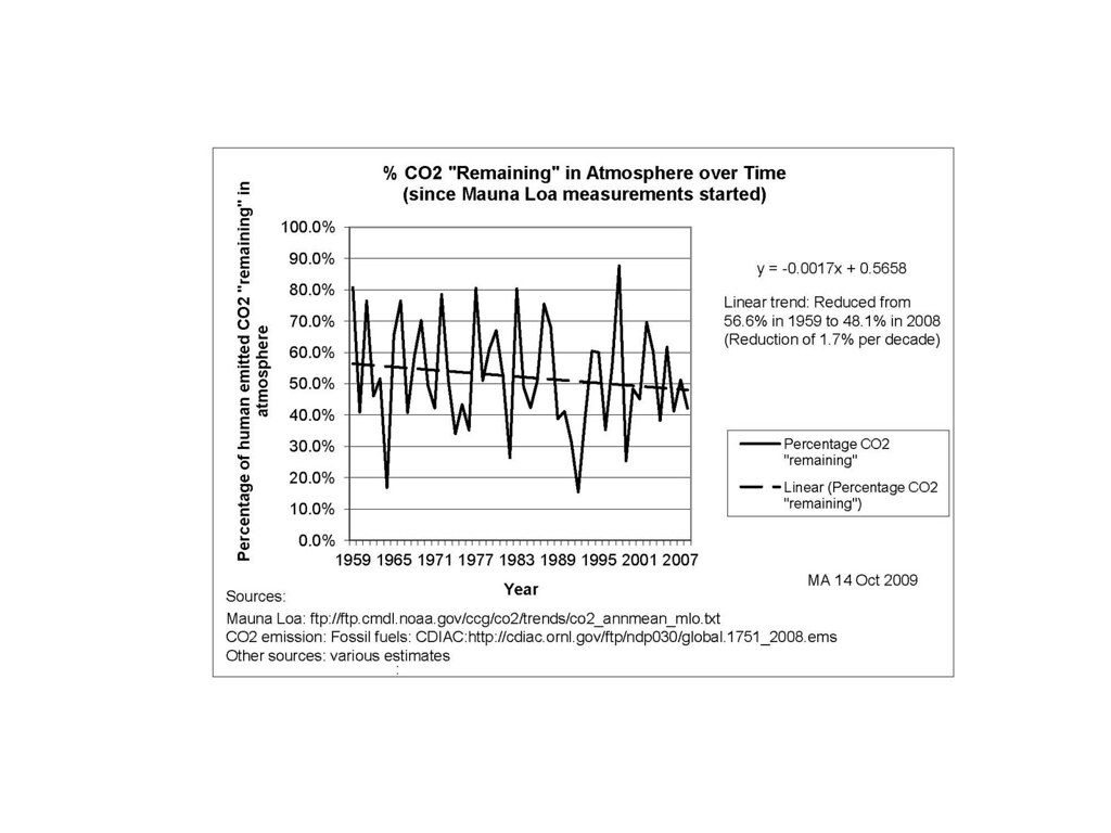
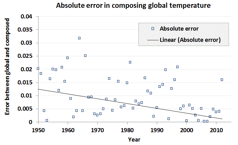
On the right is the model with the incorporation of a temperature-dependent outgassed fraction. In this case the model is more noisy than the data, as it includes outgassing of CO2 depending on the global temperature for that year. Since the temperature is noisy, the CO2 fraction picks up all of that noise.  Still, the airborne fraction shows a small yet perceptible decline, and the model matches the data well, especially in recent years where the temperature fluctuations are reduced.

Amazing that over 50 years, the mean fraction has not varied much from 55%. That has a lot to do with the math of diffusional physics. Essentially a random walk moving into and out of sequestering sites is a 50/50 proposition. That’s the way to intuit the behavior, but the math really does the heavy lifting in predicting the fraction sequestered out.

It looks like the theory matches the data once again. The skeptics provide a knee-jerk view that this behavior is not well understood, but not having done the analysis themselves, they lose out -- the skeptic meme is simply one of further propagating fear, uncertainty, and doubt (FUD) without concern for the underlying science.

Proportional Land/Sea Global Warming Model

I found an interesting global temperature regression exercise that may lead to some insight with respect to understanding ocean heat content .  From a previous post we estimated that about half the excess heat produced over the oceans is getting stored (sequestered) in the ocean depths.  The intriguing premise is that we can potentially substantiate the flow of heat by comparing the relative growths of global temperatures against the land-only temperatures and the ocean-surface temperatures (i.e. the sea-surface temperatures known as SST).

The elementary kriging approximation is that the global temperature anomaly (T_G) is a proportional mix of the ocean temperature (T_o) with the land temperature (T_l ):
$$ T_G = p_o T_o + p_l T_l $$
where
$$ 1 = p_o + p_l $$
with the approximate fraction of earth's coverage by the ocean equal to 0.7 (and the land therefore 0.3).

We use that Hadley center data sets

global	land	ocean
hadcrut4	crutem4vgl	hadsst2gl

Shifting the baseline anomaly by at most 0.1C, we come up with the following fit, shown in Figure 1.  The composed temperature lines up very closely to the reported global temperature, with the red areas peeking out where the agreement is not perfect.

Figure 1 : Global temperature anomaly is straightforwardly recreated by assuming that the global temperature is composed by a proportion of ocean and land area.  The fit works very well apart from a few points (years centered around 1948) that may be traced to systemic errors or discrepancies the database versions.

That by itself is only somewhat interesting, as it merely confirms that the Hadley center researchers know how to do first order proportional mapping (aka kriging). The regression agreement is shown in Figure 2.

Figure 2 : The composed temperature maps nearly one-to-one to the actual global temperature.

The other identity we need to consider involves a fraction of the heat sunk by the ocean. Since the land has essentially no heat sink, but that the ocean has a fraction f that acts as a heat sink, we can assert:
$$ T_o = f T_g $$
where we determined previously that f is about 0.5.

We can plot the linear regression between the two below.

Figure 3 : Linear regression between Land and SST temperature is more noisy.

As this is fit is fairly noisy, we can try to reduce the variance by plotting against the global mean temperature as a multiple regression fit.  We take the first equation and replace each of the component temperatures with their fractional equivalents.
$$ T_G =  p_o  f T_l + p_l T_l $$
$$ T_G =  p_o T_o + p_l \frac{T_o}{f}  $$
and then apply these as equal weightings
$$ T_G = 1/2 ( p_o f T_l + p_l T_l ) +  1/2 ( p_o T_o + p_l \frac{T_o}{f} )$$

rearranging terms
$$ T_G = 1/2 ( f p_o + p_l  ) T_l +  1/2 ( p_o + \frac{p_l}{f} ) T_o $$
If we apply a multiple regression of the global temperature data against a linear combination of the ocean and temperature data we get the following tabulated results:

	Coefficients	Standard Error	t Stat	P-value	Lower 95%	Upper 95%
Intercept	0.02225179	0.003884172	5.728838	4.97E-08	0.0145802	0.02992339
Land	0.29922517	0.015995888	18.70638	6.56E-42	0.26763182	0.33081852
Ocean	0.65796939	0.024637656	26.70584	1.86E-60	0.60930775	0.70663103

With this information, we can solve for f and the land ocean split.
$$ 1/2 ( f p_o + p_l  ) = 0.299 $$
$$ 1/2 ( p_o + \frac{p_l}{f} ) = 0.658 $$
Given two linear equations and two unknowns, we get f = 0.46 and ocean fraction of 73.5%.
The solution is also shown as the open circles in Figure 1.

We originally asserted that 1/2 the heat is entering the ocean, and substantiated this with a value of 0.46.  We can also compare the generally agreed upon value of 71% of the surface water coverage with the value of 73.5% determined here.  Given the confidence interval uncertainty in the coefficients as shown in the table above, we see that this simple analysis substantiates our original premise.

This is also a subtle effect and can easily be misinterpreted as arising from just the proportional warming of ocean and land. However something has to create the temperature imbalance between the ocean and land, and the fact that the coefficients of proportionality shown in the table come out fairly close to 0.3 and 0.7 (those of land and ocean) is just a coincidence in the math. If some value markedly different from 0.5 for heat sinking was involved, then the ratios would differ more obviously.

Climate science, like other science disciplines, consists of an array of interlocking parts that need to fit together. If these don't fit, our model will lose its predictive power.  In the case of this model, we can help verify that the excess heat is entering the ocean, suppressing the global temperature by about 2/3 from the land temperature.   This will continue as long as the ocean acts as a heat sink, a point still some distance in the future.   All we can really say is that global temperature anomalies have the potential for increasing by 3/2 or by 50% from the current readings when they eventually and asymptotically reach a near-equilibrium steady-state.

                                    UPDATE                                   

Using the Eureqa curve fitting software, a linear combination of data sets provides the low complexity fit.

Figure 4: The linear combination of SST and Land with an offset gives a Pareto frontier optimum

                                   It's the ocean heat content, stupid                                   

June 22, 2013. This paper has applicability to the proportional land/sea warming model

M. Watanabe, Y. Kamae, M. Yoshimori, A. Oka, M. Sato, M. Ishii, T. Mochizuki, and M. Kimoto, “Strengthening of ocean heat uptake efficiency associated with the recent climate hiatus,” Geophysical Research Letters, 2013.

The research results claim that the ocean has been adjusting its heat uptake in the last few years as a result of transient changes in the large-scale hydrodynamics.  This has the effect of suppressing the warming in terms of temperature, although the heat uptake from the AGW forcing still exists. So the implication is that what is lacking in a temperature rise is made up for by the heat sinking of the ocean  (also see the "missing heat" issue studied by Trenberth).

The ocean heat uptake efficiency measure of Watanabe is related to the ratio f between ocean and land temperature defined at the top of this post. The idea is that -- similar to the aim of the Japanese research study -- to see if we can detect changes in f over the last few years.

To do this we need to take great care with the numbers. Instead of using the WoofForTrees data, I used the CRU data directly.  The sets were CRUTEM4 (land), HadCRUT4 (global), and HadSST3 (sea).  The composed set looks like the following chart for a value of f = 0.5, which is the nominal fraction assumed for the original proportional land/sea analysis.

The composed temperature lies on top of the HadCRUT4 global temperature

If we look at the error residual between the HadCRUT4 global temperature and the fractionally composed model, we get the following chart.  Note that as an absolute error, the value is obviously decreasing over time, likely attributed to better and more accurate record keeping with current temperature measurement techniques.

The absolute error decreases with more recent records.
(The last data point is 2012, which often undergoes corrections for the next update.)

The high resolution and low error in recent years indicates that perhaps we can try to more accurately fit the fraction f.   So essentially, we want to zero out the error by solving the proportional land/sea warming model for a continuously varying value of f.
$$ 0 = T_G - 1/2 ( f p_o + p_l  ) T_l +  1/2 ( p_o + \frac{p_l}{f} ) T_o $$
This turns into a quadratic equation for f, which we can solve by the quadratic formula. The set of value calculated by minimizing the error is shown below.  Note that the average remains around f = 0.5, but it shows a distinct decreasing trend in recent years.

The fraction ratio of ocean to land temperature appears to be decreasing in recent years, leading to an apparent flattening in global temperature rise. Lower values of f cause the global temperature signal to appear cooler for a given AGW forcing.

If this is a real trend (as opposed to some type of accumulating systemic error or noise) it is telling us that more of the heat is accumulating in the ocean, consistent with the claims of Watanabe et al.   It is possible that the fraction is actually decreasing from a past value of around 0.6 to a current value of 0.4.  Although this is a subtle effect in terms of the fit (probably the not most robust metric one can imagine), it has significant effect in terms of the global surface temperature signal.

This is seen if we deconstruct the proportional model in terms of the land temperature alone, assuming the area land/ocean split as 0.71/0.29 :

$$ T_G =  (0.71 \cdot f + 0.29 ) T_l $$
Note that with a slowly increasing land temperature signal T_l , the declining f can compensate for this value and actually cause the global temperature value T_G to flatten.

To take an example, reducing the value of f from 0.6 to 0.4 causes the global temperature to decline from 0.716*T_l to 0.574*T_l.  If the land temperature is held constant, the global temperature will decline, while if the land temperature rises by 25%, the global temperature rise will look flat.

Contour plot showing optimal values of f.  This is a log plot and higher negative values indicate low error

That is exactly what Watanabe et al are claiming.  Moreover, they assert that this decline can't remain in place for the long term, and eventually the ocean hydrodynamics will stabilize or even reverse, with a concomitant rebound in global temperature.

To review, the essential premise of the proportional land/ocean model is:

1. The land surface reaches the steady-state temperature quickly
2. The ocean sinks excess heat, thus moderating the sea surface temperature rise.
3. The fractional ratio of ocean temperature to land temperature is given by f.
4. The global surface temperature is determined as combination of land and sea surface temperatures prorated according to the land/sea areal split.

From this set of premises, we can algebraically estimate the amount of ocean heat sinking from global temperature records as gleaned from the Climatic Research Unit.

(also see I. Held's blog post on this topic [2])

References

[1]

D. Dommenget, “The ocean’s role in continental climate variability and change,” Journal of Climate, vol. 22, no. 18, pp. 4939–4952, 2009.

“The land–sea warming ratio in the ECHAM–HadISST holds also for the warming trend over the most recent decades, despite the fact that no anthropogenic radiative forcings are included in the simulations. The temperature trends during the past decades as observed and in the (ensemble mean) model response (Fig. 4) are roughly consistent with each other, which indicates that much of the land warming is a response to the warming of the oceans. The simulated land warming, however, is weaker than that observed in many regions, with an average land–sea warming ratio of 1.6, amounting to about 75% of the observed ratio of 2.1 .”

[2]

I. Held, “38. NH-SH differential warming and TCR « Isaac Held’s Blog.” [Online]. Available: http://www.gfdl.noaa.gov/blog/isaac-held/2013/06/14/38-nh-sh-differential-warming-and-tcr/#more-5774. [Accessed: 25-Jun-2013].

Greenland Red Noise

Tamino analyzed a paper by Chylek [1] who claimed to be able to extract a periodic signal out of Greenland ice core data (Dye3).

Tamino's post is comprehensive, but I wanted to check to see if I could extract any signal from the data myself.

The data is in the upper right of the following figure, and the FFT-based power spectral density (PSD) is in the lower left. 

FFT PSD lower left, Data upper right

The PSD is nondescript with a red noise envelope shown by the solid line. Red noise is the embodiment of the Ornstein-Uhlenbeck process.  This red noise shows very short correlation, at most a lag of one or two time units, as shown in the autocorrelation below.

Autocorrelation function, centered at 1/2 time series length

Hard pressed to find any real signal in such a time series.  A simulation of Ornstein-Uhlenbeck red noise is shown to the left below, with a slice of the Greenland data to the right.

Ornstein-Uhlenbeck red noise time series (left) and slice of data (right)

Chylek claims that he can see 20 year AMO (Atlantic Ocean) oscillations in the data. Like Tamino, I see nothing but garden variety noise.


References

[1]

P. Chylek, C. Folland, L. Frankcombe, H. Dijkstra, G. Lesins, and M. Dubey, “Greenland ice core evidence for spatial and temporal variability of the Atlantic Multidecadal Oscillation,” Geophysical Research Letters, vol. 39, no. 9, 2012.

 

 

Filtering Sea Level Rise

Measuring global sea-level rise is not for the faint-of-heart.  The levels are averaged over the earth's oceans and likely are processed to remove tidal and other effects.

At one of the climate blogs, a gang of climate change skeptics tried to convince their fellow skeptics that the sea level rise had turned the tide (so to speak) and started to decrease. The skeptic Rob (Ringo) Starkey kindly provided the data and pointed to a recent dip in the data:

http://sealevel.colorado.edu/files/2013_rel3/sl_ns_global.txt

BDD smelled something fishy and pointed out that these are at best seasonal dips and labelled it rubbish, and reasoned that they were likely trying to save face over some other wrong they had committed.  What I usually find is that the more that the fake skeptics howl about something, the more likely that there are creepy crawly things they are trying to hide under the rock. Well, in this case the sea-level rise data that Ringo pointed us to shows a clear 2 month oscillation in the time series. Sorry Ringo, "steven", and Captain Tuna, easy enough to put a 2-month notch filter in the time series data and just look at how much smoother it gets.
 

Figure 1 : Upper left inset is a FFT of the detrended sea-level rise data shown in the lower right inset. A clear two month cycle shows up in the FFT and by eyeballing any yearly interval.  After performing a simple 2 month notch filter on the data and adding back in the trend, the red curve shows significant noise reduction.

The oscillation is possibly identified as a meridional current fluctuation of 2 months located in the Pacific described by this Woods Hole investigation:  "Air-Sea Interaction in the Eastern Tropical Pacific ITCZ/Cold Tongue Complex" page. It also is described by a member of the same team in this PhD thesis [1] :

"The period of the oscillations can be seen to be about two months from October 1997 to June 1998, and the oscillations rapidly intensify during the first few months of 1998. The amplitude of the oscillations approximately doubles between December 1997 and February 1998, and it doubles again between February and April 1998. At its peak strength in April 1998, the signal is associated with nearly a 7 cm peak-to-peak change in the thickness of the upper 110 m of the water column. "

One can see the peaks in late 1997 and early 1998 from Figure 1, enlarged and highlighted below

Figure 2: Identification of water column thickness increase

The main point is that these fluctuations are oscillatory and don't contribute to a persistent rise in the sea-level. Like tides, this phenomena is more similar to the sloshing of water in a bucket.  (This particular two month cycle is not a tide as lunar tides such as neap and spring tides have monthly or biweekly periods).

References

[1]

J. Farrar, “Air-sea interaction at contrasting sites in the Eastern Tropical Pacific : mesoscale variability and atmospheric convection at 10°N,” PhD Thesis, MIT, Woods Hole, 2007.
http://dspace.mit.edu/handle/1721.1/39009

                                           EDIT                                                 

I noticed that the sea level research group at U of Colorado had already placed a 60 day (2 month) smoothing filter when they display the data (see figure below). This is similar to the 2-point notch filter that I use, which I set specifically to pair up data points so that they are out-of-phase at the 30-day mark.  A general smoothing filter will accomplish the same thing but will also filter out shorter periods in the data set.

http://sealevel.colorado.edu/content/2013rel3-global-mean-sea-level-time-series-seasonal-signals-removed

The Rise and Decline of UK Crude Oil

This is updated information from 2005 and 2008 concerning projections of North Sea UK Oil production. 

The following Figure 1 is a screenshot of an interactive oil shock model session, which is part of a larger environmental modeling framework. 

Figure 1:  Shock Model for UK North Sea Oil. The oil production output is the profile with two humps, with model and data shown together. Extraction rate applied to the extrapolated reserves gives the production.

The discovery curve follows a dispersive profile which allows us to project future availability along a declining tail.  The extraction perturbations show a temporary glitch corresponding to the Piper Alpha platform disaster, but otherwise shows around a 6% extraction rate from reserves over the years.  This rate isn't expected to move upwards much (contrary to my previous projection) because any increase in technological advancements will be compensated by fields that are tougher to extract from.

Also included in the interactive session is an ability to pull up individual fields (all part of a semantic web server), shown in Figure 2.  The "Forties" oil field is one of the earliest discoveries and commenced production at the start of the UK North Sea era.

Figure 2:  Individual plot of a UK platform, the "Forties" oil field. The downward glitch at the end is a -1 value indicating production values are not yet available for that year.

The UK Prime Ministers during this time (see Figure 3) likely benefited politically from the oil production bonanza, starting with Margaret Thatcher's leadership of the conservative party in 1975.

Figure 3: PM Margaret Thatcher was at the right place at the right time. Leader of the conservative party starting in 1975, and then became Prime Minister in 1979, she reigned during the huge buildup in oil production, which was temporarily halted by the Piper Alpha explosion in 1988.

The Piper production halted for several years and pulled down other platform production levels as better maintenance policies were instituted. This had the unintended benefit of extending the UK production level before the eventual decline set in.

Figure 4: Piper Alpha oil production halted for several years

As I have always said, having good numbers for production data allows use to apply sophisticated analyses such as the oil shock model to project and predict future trends. The UK government has done a fine job in making the data publicly available, allowing lots of interesting analysis which I documented in The Oil Conundrum book.

                                            Updates                                         

Feedback from others
http://www.theoildrum.com/node/9946#comment-958176
http://transportblog.co.nz/2013/04/12/oil-dependancy-and-the-wealth-of-nations/

Sources
http://www.worldreview.info/content/uk-north-sea-oil-and-gas-resurgence-activity

Ornstein-Uhlenbeck Diffusion

The Ornstein-Uhlenbeck correction to diffusion can be used in applications ranging from modeling Bakken oil production to modeling CO2 sequestration.

Due to its origins as a random walk process, a pure diffusion model of particles will show unbounded excursions given a long enough time duration. This is characterized by the unbounded Fickian growth law showing a t dependence for a pure random walk with a single diffusivity.

In practice, the physical environment of a particle may prevent unbounded excursions. It is physically possible that the environment may impose limiting effects on the extent of motion, or that it will place some form of drag on the particle’s hopping rate the further it moves away from a mean starting value.

The rationale for this limiting process within a producing hydrofractured reservoir may arise from a barrier to diffusion beyond a certain range.

Figure 1: The Ornstein-Uhlenbeck process suppresses the diffusional flow by limiting the extent at which the mobile solute can travel, thus generating a constrained asymptote below that of drag-free diffusion.

Similarly, a sequestration barrier may exist preventing CO2 from permanently exiting the active carbon cycle; this makes the fat temporal tail even fatter.

Figure 2 : Impulse Response of the sequestering of Carbon Dioxide to a normalized stimulus. The solid blue curve represents the generally accepted model, while the dashed and dotted curves represent the dispersive diffusion model with O-U correction. The correction flattens out the tail.

We can use the Ornstein-Uhlenbeck process to model mathematically how this pure random walk becomes bounded. The Ornstein-Uhlenbeck process has its origins in the modeling of Brownian motion with a special “reversion to the mean” property in motion excursions (specifically, it was first formulated to describe Brownian motion in the presence of drag on particle velocities, extending Einstein's work). The following expression shows the stationary marginal probability given a stochastic differential equation

dX=-a X∙dt+dW

which models a drag on an excursion [1]

dPXt+s=x Xs= 0)= 12πτe-x22τ dx 

where τ=1-e-2at2a

The O-U correction is straight-forward to apply on our dispersive growth formulation, we only need apply a non-linear transformation to the time-scale.

t →O-Uτ

and then apply this to a dispersive growth term such as the following:

xτ(t)=Dτ(t)Dτ(t)x01+ Dτ(t)x0 →where τt=(1-e-2at)/2a

This has the equivalent effect of appearing to slow down time at an exponential rate. This exponential rate turns out to be much faster than the Fickian growth law can sustain, so that an asymptotic limit is achieved in the diffusional growth extent.

Figure 3: The reversion to the mean process of the Ornstein-Uhlenbeck process will limit the growth of a diffusional process

A physical model of an attractor or potential well which “tugs” on the random walker to bring it back to the mean state (see Figure below).

Figure 4: Representation of an Ornstein-Uhlenbeck random walk process. The hopping rate works similarly to a potential well, with a greater resistance to hopping the further excursion ways from the mean.

Algorithmic Code

The following pseudo-code snippet sets up an Ornstein-Uhlenbeck random walk model with a reversion-to-the-mean term. The diffusion term is the classical Markovian random walk transition rate. The drag term places an attractor which opposes large excursions in the term Z.

-- Ornstein-Uhlenbeck random walk = ou

ou(X1, X2, Z)
   random(R)
   if R < 0.5 then
      Z = Z*X1 + X2
   else
      Z = Z*X1 - X2
   end

-- This is how it gets parameterized

ou_random_walker (dX, Diffusion, Drag, Z)
   X1 = exp(-2*Drag*dX)
   X2 = sqrt(Diffusion*(1-exp(-2*Drag*dX))/2/Drag)
   ou(X1, X2, Z)

Variance

To determine whether an Ornstein-Uhlenbeck process is apparent on a set of data, one can apply a simple multiscale variance to the result of a Z array of length N :

variance(Z,N) {
   L = N/2
   while(L > 1) {
      Sum = 0.0
      for(i=1; i<N/2; i++) {
        Val = Z[i] - Z[i+L]
        Sum += Val * Val
      }
      print L “ “ sqrt(Sum/(N/2))
      L = 0.95*L;
   }
}

So that for a given random walk simulation, the asymptotic variance will tend to saturate at longer correlation length scales. A typical multiscale variance plot will look like those described here: http://theoilconundrum.blogspot.com/2011/11/multiscale-variance-analysis-and.html.

Autocorrelation and Spectral Representation

The autocorrelation of the Ornstein-Uhlenbeck process is, where Theta=Drag:

Rx= Dθ e-θ|x|

Even though this shows a saturation level, the power spectrum still obeys a 1/S^2 fall-off.

ISx= Dπ∙1Sx2+θ2

The Orenstein-Uhlenbeck process is often referred to as red noise and the two parameters of Diffusion and Drag can be determined either from the autocorrelation function or from the PSD. For the PSD, on a log-log plot, this involves reading the peak near S=0 and then determining the shoulder of the power-law roll-off. Between these two measures, one can infer both parameter values.

References

[1]

D. Mumford and A. Desolneux, Pattern Theory: The Stochastic Analysis Of Real-World Signals. A K Peters, Ltd., 2010.