Context/Earth

[[ Check out my Wordpress blog Context/Earth for environmental and energy topics tied together in a semantic web framework ]]


Sunday, April 28, 2013

Greenland Red Noise

Tamino analyzed a paper by Chylek [1] who claimed to be able to extract a periodic signal out of Greenland ice core data (Dye3).

Tamino's post is comprehensive, but I wanted to check to see if I could extract any signal from the data myself.

The data is in the upper right of the following figure, and the FFT-based power spectral density (PSD) is in the lower left. 

FFT PSD lower left, Data upper right

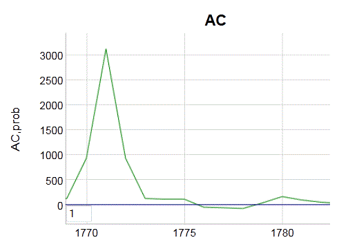
The PSD is nondescript with a red noise envelope shown by the solid line. Red noise is the embodiment of the Ornstein-Uhlenbeck process.  This red noise shows very short correlation, at most a lag of one or two time units, as shown in the autocorrelation below.

Autocorrelation function, centered at 1/2 time series length

Hard pressed to find any real signal in such a time series.  A simulation of Ornstein-Uhlenbeck red noise is shown to the left below, with a slice of the Greenland data to the right.
Ornstein-Uhlenbeck red noise time series (left) and slice of data (right)
Chylek claims that he can see 20 year AMO (Atlantic Ocean) oscillations in the data. Like Tamino, I see nothing but garden variety noise.


References

[1]
P. Chylek, C. Folland, L. Frankcombe, H. Dijkstra, G. Lesins, and M. Dubey, “Greenland ice core evidence for spatial and temporal variability of the Atlantic Multidecadal Oscillation,” Geophysical Research Letters, vol. 39, no. 9, 2012.


Wednesday, April 24, 2013

Filtering Sea Level Rise

Measuring global sea-level rise is not for the faint-of-heart.  The levels are averaged over the earth's oceans and likely are processed to remove tidal and other effects.

At one of the climate blogs, a gang of climate change skeptics tried to convince their fellow skeptics that the sea level rise had turned the tide (so to speak) and started to decrease. The skeptic Rob (Ringo) Starkey kindly provided the data and pointed to a recent dip in the data:
http://sealevel.colorado.edu/files/2013_rel3/sl_ns_global.txt
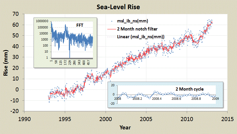
BDD smelled something fishy and pointed out that these are at best seasonal dips and labelled it rubbish, and reasoned that they were likely trying to save face over some other wrong they had committed.  What I usually find is that the more that the fake skeptics howl about something, the more likely that there are creepy crawly things they are trying to hide under the rock. Well, in this case the sea-level rise data that Ringo pointed us to shows a clear 2 month oscillation in the time series. Sorry Ringo, "steven", and Captain Tuna, easy enough to put a 2-month notch filter in the time series data and just look at how much smoother it gets.
 
Figure 1 : Upper left inset is a FFT of the detrended sea-level rise data shown in the lower right inset. A clear two month cycle shows up in the FFT and by eyeballing any yearly interval.  After performing a simple 2 month notch filter on the data and adding back in the trend, the red curve shows significant noise reduction.

The oscillation is possibly identified as a meridional current fluctuation of 2 months located in the Pacific described by this Woods Hole investigation:  "Air-Sea Interaction in the Eastern Tropical Pacific ITCZ/Cold Tongue Complex" page. It also is described by a member of the same team in this PhD thesis [1] :
"The period of the oscillations can be seen to be about two months from October 1997 to June 1998, and the oscillations rapidly intensify during the first few months of 1998. The amplitude of the oscillations approximately doubles between December 1997 and February 1998, and it doubles again between February and April 1998. At its peak strength in April 1998, the signal is associated with nearly a 7 cm peak-to-peak change in the thickness of the upper 110 m of the water column. "
One can see the peaks in late 1997 and early 1998 from Figure 1, enlarged and highlighted below

Figure 2: Identification of water column thickness increase
The main point is that these fluctuations are oscillatory and don't contribute to a persistent rise in the sea-level. Like tides, this phenomena is more similar to the sloshing of water in a bucket.  (This particular two month cycle is not a tide as lunar tides such as neap and spring tides have monthly or biweekly periods).

References

[1]
J. Farrar, “Air-sea interaction at contrasting sites in the Eastern Tropical Pacific : mesoscale variability and atmospheric convection at 10°N,” PhD Thesis, MIT, Woods Hole, 2007.
http://dspace.mit.edu/handle/1721.1/39009


                                           EDIT                                                 


I noticed that the sea level research group at U of Colorado had already placed a 60 day (2 month) smoothing filter when they display the data (see figure below). This is similar to the 2-point notch filter that I use, which I set specifically to pair up data points so that they are out-of-phase at the 30-day mark.  A general smoothing filter will accomplish the same thing but will also filter out shorter periods in the data set.


http://sealevel.colorado.edu/content/2013rel3-global-mean-sea-level-time-series-seasonal-signals-removed


Saturday, April 20, 2013

The Rise and Decline of UK Crude Oil


This is updated information from 2005 and 2008 concerning projections of North Sea UK Oil production. 

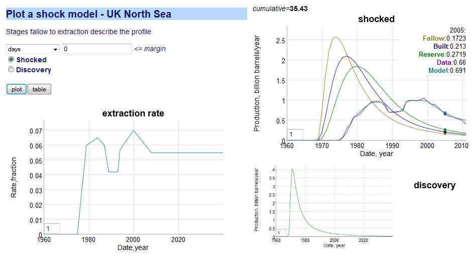
The following Figure 1 is a screenshot of an interactive oil shock model session, which is part of a larger environmental modeling framework. 

Figure 1:  Shock Model for UK North Sea Oil. The oil production output is the profile with two humps, with model and data shown together. Extraction rate applied to the extrapolated reserves gives the production.

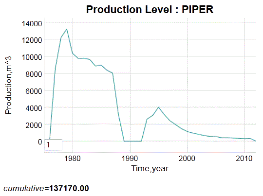
The discovery curve follows a dispersive profile which allows us to project future availability along a declining tail.  The extraction perturbations show a temporary glitch corresponding to the Piper Alpha platform disaster, but otherwise shows around a 6% extraction rate from reserves over the years.  This rate isn't expected to move upwards much (contrary to my previous projection) because any increase in technological advancements will be compensated by fields that are tougher to extract from.

Also included in the interactive session is an ability to pull up individual fields (all part of a semantic web server), shown in Figure 2.  The "Forties" oil field is one of the earliest discoveries and commenced production at the start of the UK North Sea era.

Figure 2:  Individual plot of a UK platform, the "Forties" oil field. The downward glitch at the end is a -1 value indicating production values are not yet available for that year.
The UK Prime Ministers during this time (see Figure 3) likely benefited politically from the oil production bonanza, starting with Margaret Thatcher's leadership of the conservative party in 1975.

Figure 3: PM Margaret Thatcher was at the right place at the right time. Leader of the conservative party starting in 1975, and then became Prime Minister in 1979, she reigned during the huge buildup in oil production, which was temporarily halted by the Piper Alpha explosion in 1988.


The Piper production halted for several years and pulled down other platform production levels as better maintenance policies were instituted. This had the unintended benefit of extending the UK production level before the eventual decline set in.
Figure 4: Piper Alpha oil production halted for several years
As I have always said, having good numbers for production data allows use to apply sophisticated analyses such as the oil shock model to project and predict future trends. The UK government has done a fine job in making the data publicly available, allowing lots of interesting analysis which I documented in The Oil Conundrum book.


                                            Updates                                         

Feedback from others
http://www.theoildrum.com/node/9946#comment-958176
http://transportblog.co.nz/2013/04/12/oil-dependancy-and-the-wealth-of-nations/

Sources
http://www.worldreview.info/content/uk-north-sea-oil-and-gas-resurgence-activity


Thursday, April 18, 2013

Ornstein-Uhlenbeck Diffusion

The Ornstein-Uhlenbeck correction to diffusion can be used in applications ranging from modeling Bakken oil production to modeling CO2 sequestration.

Due to its origins as a random walk process, a pure diffusion model of particles will show unbounded excursions given a long enough time duration. This is characterized by the unbounded Fickian growth law showing a t dependence for a pure random walk with a single diffusivity.

In practice, the physical environment of a particle may prevent unbounded excursions. It is physically possible that the environment may impose limiting effects on the extent of motion, or that it will place some form of drag on the particle’s hopping rate the further it moves away from a mean starting value.

The rationale for this limiting process within a producing hydrofractured reservoir may arise from a barrier to diffusion beyond a certain range.

Figure 1: The Ornstein-Uhlenbeck process suppresses the diffusional flow by limiting the extent at which the mobile solute can travel, thus generating a constrained asymptote below that of drag-free diffusion.


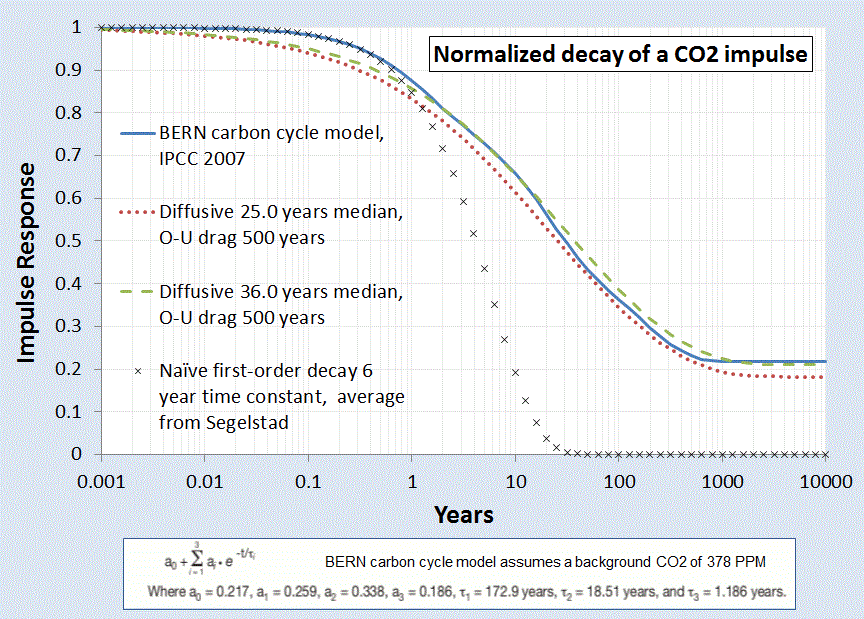
Similarly, a sequestration barrier may exist preventing CO2 from permanently exiting the active carbon cycle; this makes the fat temporal tail even fatter.

Figure 2 : Impulse Response of the sequestering of Carbon Dioxide to a normalized stimulus. The solid blue curve represents the generally accepted model, while the dashed and dotted curves represent the dispersive diffusion model with O-U correction. The correction flattens out the tail.


We can use the Ornstein-Uhlenbeck process to model mathematically how this pure random walk becomes bounded. The Ornstein-Uhlenbeck process has its origins in the modeling of Brownian motion with a special “reversion to the mean” property in motion excursions (specifically, it was first formulated to describe Brownian motion in the presence of drag on particle velocities, extending Einstein's work). The following expression shows the stationary marginal probability given a stochastic differential equation

dX=-a Xdt+dW

which models a drag on an excursion [1]
dPXt+s=x  Xs= 0)= 12πτe-x22τ dx 
where   τ=1-e-2at2a


The O-U correction is straight-forward to apply on our dispersive growth formulation, we only need apply a non-linear transformation to the time-scale.

t O-Uτ


and then apply this to a dispersive growth term such as the following:


xτ(t)=Dτ(t)Dτ(t)x01+ Dτ(t)x0    where    τt=(1-e-2at)/2a  


This has the equivalent effect of appearing to slow down time at an exponential rate. This exponential rate turns out to be much faster than the Fickian growth law can sustain, so that an asymptotic limit is achieved in the diffusional growth extent.

Figure 3: The reversion to the mean process of the Ornstein-Uhlenbeck process will limit the growth of a diffusional process


A physical model of an attractor or potential well which “tugs” on the random walker to bring it back to the mean state (see Figure below).

Figure 4: Representation of an Ornstein-Uhlenbeck random walk process. The hopping rate works similarly to a potential well, with a greater resistance to hopping the further excursion ways from the mean.

Algorithmic Code


The following pseudo-code snippet sets up an Ornstein-Uhlenbeck random walk model with a reversion-to-the-mean term. The diffusion term is the classical Markovian random walk transition rate. The drag term places an attractor which opposes large excursions in the term Z.


-- Ornstein-Uhlenbeck random walk = ou

ou(X1, X2, Z)
   random(R)
   if R < 0.5 then
      Z = Z*X1 + X2
   else
      Z = Z*X1 - X2
   end


-- This is how it gets parameterized

ou_random_walker (dX, Diffusion, Drag, Z)
   X1 = exp(-2*Drag*dX)
   X2 = sqrt(Diffusion*(1-exp(-2*Drag*dX))/2/Drag)
   ou(X1, X2, Z)

Variance

To determine whether an Ornstein-Uhlenbeck process is apparent on a set of data, one can apply a simple multiscale variance to the result of a Z array of length N :

variance(Z,N) {
   L = N/2
   while(L > 1) {
      Sum = 0.0
      for(i=1; i<N/2; i++) {
        Val = Z[i] - Z[i+L]
        Sum += Val * Val
      }
      print L “ “ sqrt(Sum/(N/2))
      L = 0.95*L;
   }
}


So that for a given random walk simulation, the asymptotic variance will tend to saturate at longer correlation length scales. A typical multiscale variance plot will look like those described here: http://theoilconundrum.blogspot.com/2011/11/multiscale-variance-analysis-and.html.

Autocorrelation and Spectral Representation

The autocorrelation of the Ornstein-Uhlenbeck process is, where Theta=Drag:

Rx= Dθ e-θ|x|

Even though this shows a saturation level, the power spectrum still obeys a 1/S^2 fall-off.

ISx= Dπ1Sx2+θ2


The Orenstein-Uhlenbeck process is often referred to as red noise and the two parameters of Diffusion and Drag can be determined either from the autocorrelation function or from the PSD. For the PSD, on a log-log plot, this involves reading the peak near S=0 and then determining the shoulder of the power-law roll-off. Between these two measures, one can infer both parameter values.

References


[1]
D. Mumford and A. Desolneux, Pattern Theory: The Stochastic Analysis Of Real-World Signals. A K Peters, Ltd., 2010.


Thursday, March 28, 2013

Ocean Heat Content Model

The ocean heat content continues to increase and perhaps accelerate [1], as expected due to global warming. In an earlier post, I analyzed the case of the "missing heat", which wasn't missing after all, but the result of the significant heat sinking characteristics of the oceans [2].

The objective is to create a simple model which tracks the transient growth as shown in the recent paper by Balmaseda, Trenberth, and Källén (BTK)[1] and described in Figure 1 below

Figure 1: Ocean Heat Content from BTK [1] (source)
We will assume a diffusive flow of heat as described in James Hansen’s 1981 paper [2]. In general  the diffusion of heat is qualitatively playing out according to the way Fick’s law would apply to a heat sink. Hansen also volunteered an effective diffusion that should apply, set to the nice round number of 1 cm^2/second.

In the following we provide a mathematical explanation which works its way from first principles to come up with an uncertainty-quantified formulation. After that we present a first-order sanity check to the approximation.

Solution

We have three depths that we are looking at for heat accumulation (in addition to a surface layer which gives only a sea-surface temperature or SST). These are given as depths to 300 meters, to 700 meters, and down to infinity (or 2000 meters from another source), as charted on Figure 1.

We assume that excess heat (mostly infrared) is injected through the ocean's surface and works its way down through the depths by an effective diffusion coefficient.  The kernel transient solution to the planar heat equation is this:

$$\Delta T(x,t) = \frac{c}{\sqrt{D_i t}} \exp{\frac{-x^2}{D_i t}} $$
where D_i is the diffusion coefficient, and x is the depth (note that often a value of 2D instead of D is used depending on the definition of the random walk).  The delta temperature is related to a thermal energy or heat through the heat capacity of salt water, which we assume to be constant through the layers. Any scaling is accommodated by the prefactor, c

The first level of uncertainty is a maximum entropy prior (MaxEnt) that we apply to the diffusion coefficient to approximate the various pathways that heat can follow downward.  For example, some of the flow will be by eddy diffusion and other paths by conventional vertical mixing diffusion.  If we apply a maximum entropy probability density function, assuming only a mean value for the diffusion coefficient:
$$ p(D_i) = \frac{1}{D} e^{\frac{-D_i}{D}} $$

then we get this formulation:
$$\Delta T(t|x) = \frac{c}{\sqrt{D t}} e^{\frac{-x}{\sqrt{D t}}} (1 + \frac{x}{\sqrt{D t}})$$

The next uncertainty is in capturing the heat content for a layer. The incremental heat across a layer, L, we can approximate as
$$ \int { \Delta T(t|x) p(x) dx}  = \int { \Delta T(t|x) e^{\frac{-x}{L}} dx} $$

Which gives as the excess heat response the following concise equation.
$$ I(t) = \frac{ \frac{\sqrt{Dt}}{L} + 2 }{(\frac{\sqrt{Dt}}{L} + 1)^2}$$

This is also the response to a delta forcing impulse, but for a realistic situation where a growing aCO2 forces the response (explained in the previous post), we simply apply a convolution of the thermal stimulus with the thermal response.  The temporal profile of the increasing aCO2 generates a growing thermal forcing function.

$$ R(t) = F(t) \otimes I(t) = \int_0^t { F(\tau) I(t-\tau) d\tau} $$
If the thermal stimulus is a linearly growing heat flux, which roughly matches the GHG forcing function (see Figure 7 in the previous post)
 $$ F(t) = k \cdot (t-t_0) $$
then assuming a starting point t_0=0.
$$ R(t)/k = \frac{2 L}{3} {(D t)}^{1.5}- L^2 D t+2 L^3 \sqrt{D t}-2 L^4 \ln(\frac{\sqrt{D t}+L}{L})) $$

A good approximation is to assume the thermal forcing function started kicking in about 50 years ago, circa1960. We can then plot the equation for various values of the layer thickness, L, and a value of D of 3 cm^2/s.
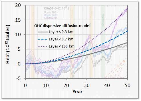
Figure 2 : Thermal Dispersive Diffusion Model applied to the OHC data

Another view of the OHC includes the thermal mass of the non-ocean regions (see Figure 3). This data appears smoothed in comparison to the raw data of Figure 2.

Figure 3 :  Alternate view of growing ocean heat content. This also includes non-ocean.
In the latter figure, the agreement with the uncertainty-quantified theory is more striking. A single parameter, Hansen's effective diffusion coefficient D, along with the inferred external thermal forcing function is able to reproduce the temporal profile accurately.

The strength of this modeling approach is to lean on the maximum entropy principle to fill in the missing gaps where the variability in the numbers are uncertain.  In this case, the diffusion and ocean depths hold the uncertainty, and we use first-order phyiscs to do the rest.


Sanity Check

The following is a sanity check for the above formulation; providing essentially a homework assignment that a physics professor would hand out in class.

An application of Fick’’s Law is to approximate the amount of material that has diffused (with thermal diffusion coefficient D) at least a certain distance, x, over a time duration, t, by

$$ e^{\frac{-x}{\sqrt{Dt}}}= \frac{Q}{Q_0}$$
  • For greater than 300 meters, Q/Q_0 is 13.5/20 read from Figure 1.
  • For greater than 700 meters, Q/Q_0 is 7.5/20
Where Q_0=20 is the baseline for the total heat measured over all depths (i.e. between x=0 and x=infinite depth) reached at the current time. No heat will diffuse to infinite depths so at that point Q/Q_0 is 0/20.

First, we can check to see how close the value of L=sqrt(Dt) scales, by fitting the Q/Q_0 ratio at each depth..
  • For x=300 meters, we get L=763
  • For x=700 meters, we get L=713
These two are close enough to maintaining invariance that the Fick’’s law scaling relation holds and we can infer that the flow is by an effective diffusion, just as was surmised by Hansen et al in 1981.

We then use an average elapsed diffusion time of t=40 years and assume an average diffusion depth of 740, and D comes out to 4.5 cm^2/s.

Hansen in 1981 [2] used an estimated value of diffusion of 1 cm^2/s, which is within an order of magnitude of 4.5 cm^2/s

This is a scratch attempt at an approximate solution to the more general solution, which is the equivalent of generating an impulse function in the past and watching that evolve. The general solution which we formulated earlier involves a modulated forcing function and we compute the convolution against the thermal impulse response (i.e. Green’s function) and compare that against Figure 1 and Figure 2, and the full temporal profile.

Discussion

Reading Hansen and looking at the BTK paper’s results, we should note that nothing looks out of the ordinary for the OHC trending if we compare it to what conventional thermal physics would predict. The total heat absorbed by the ocean is within  range of that expected by a 3C doubling sensitivity. BTK has done the important step in determining the amount of total heat absorbed, which allows us to estimate the effective diffusion coefficient by evaluating how the heat contents modulate with depth.We add a maximum uncertainty modifier to the coefficient to model the disorder in diffusivity (some of it eddy diffusivity, some vertical, etc) and that allows us to match the temporal profile accurately.


References

[1]
M. A. Balmaseda, K. E. Trenberth, and E. Källén, “Distinctive climate signals in reanalysis of global ocean heat content,” Geophysical Research Letters, 2013.


[2]
J. Hansen, D. Johnson, A. Lacis, S. Lebedeff, P. Lee, D. Rind, and G. Russell, “Climate impact of increasing atmospheric carbon dioxide,” Science, vol. 213 (4511), pp. 957–966.
http://pubs.giss.nasa.gov/docs/1981/1981_Hansen_etal.pdf