Ornstein-Uhlenbeck Diffusion

The Ornstein-Uhlenbeck correction to diffusion can be used in applications ranging from modeling Bakken oil production to modeling CO2 sequestration.

Due to its origins as a random walk process, a pure diffusion model of particles will show unbounded excursions given a long enough time duration. This is characterized by the unbounded Fickian growth law showing a t dependence for a pure random walk with a single diffusivity.

In practice, the physical environment of a particle may prevent unbounded excursions. It is physically possible that the environment may impose limiting effects on the extent of motion, or that it will place some form of drag on the particle’s hopping rate the further it moves away from a mean starting value.

The rationale for this limiting process within a producing hydrofractured reservoir may arise from a barrier to diffusion beyond a certain range.

Figure 1: The Ornstein-Uhlenbeck process suppresses the diffusional flow by limiting the extent at which the mobile solute can travel, thus generating a constrained asymptote below that of drag-free diffusion.

Similarly, a sequestration barrier may exist preventing CO2 from permanently exiting the active carbon cycle; this makes the fat temporal tail even fatter.

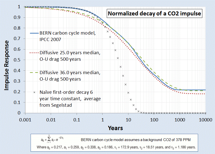
Figure 2 : Impulse Response of the sequestering of Carbon Dioxide to a normalized stimulus. The solid blue curve represents the generally accepted model, while the dashed and dotted curves represent the dispersive diffusion model with O-U correction. The correction flattens out the tail.

We can use the Ornstein-Uhlenbeck process to model mathematically how this pure random walk becomes bounded. The Ornstein-Uhlenbeck process has its origins in the modeling of Brownian motion with a special “reversion to the mean” property in motion excursions (specifically, it was first formulated to describe Brownian motion in the presence of drag on particle velocities, extending Einstein's work). The following expression shows the stationary marginal probability given a stochastic differential equation

dX=-a X∙dt+dW

which models a drag on an excursion [1]

dPXt+s=x Xs= 0)= 12πτe-x22τ dx 

where τ=1-e-2at2a

The O-U correction is straight-forward to apply on our dispersive growth formulation, we only need apply a non-linear transformation to the time-scale.

t →O-Uτ

and then apply this to a dispersive growth term such as the following:

xτ(t)=Dτ(t)Dτ(t)x01+ Dτ(t)x0 →where τt=(1-e-2at)/2a

This has the equivalent effect of appearing to slow down time at an exponential rate. This exponential rate turns out to be much faster than the Fickian growth law can sustain, so that an asymptotic limit is achieved in the diffusional growth extent.

Figure 3: The reversion to the mean process of the Ornstein-Uhlenbeck process will limit the growth of a diffusional process

A physical model of an attractor or potential well which “tugs” on the random walker to bring it back to the mean state (see Figure below).

Figure 4: Representation of an Ornstein-Uhlenbeck random walk process. The hopping rate works similarly to a potential well, with a greater resistance to hopping the further excursion ways from the mean.

Algorithmic Code

The following pseudo-code snippet sets up an Ornstein-Uhlenbeck random walk model with a reversion-to-the-mean term. The diffusion term is the classical Markovian random walk transition rate. The drag term places an attractor which opposes large excursions in the term Z.

-- Ornstein-Uhlenbeck random walk = ou

ou(X1, X2, Z)
   random(R)
   if R < 0.5 then
      Z = Z*X1 + X2
   else
      Z = Z*X1 - X2
   end

-- This is how it gets parameterized

ou_random_walker (dX, Diffusion, Drag, Z)
   X1 = exp(-2*Drag*dX)
   X2 = sqrt(Diffusion*(1-exp(-2*Drag*dX))/2/Drag)
   ou(X1, X2, Z)

Variance

To determine whether an Ornstein-Uhlenbeck process is apparent on a set of data, one can apply a simple multiscale variance to the result of a Z array of length N :

variance(Z,N) {
   L = N/2
   while(L > 1) {
      Sum = 0.0
      for(i=1; i<N/2; i++) {
        Val = Z[i] - Z[i+L]
        Sum += Val * Val
      }
      print L “ “ sqrt(Sum/(N/2))
      L = 0.95*L;
   }
}

So that for a given random walk simulation, the asymptotic variance will tend to saturate at longer correlation length scales. A typical multiscale variance plot will look like those described here: http://theoilconundrum.blogspot.com/2011/11/multiscale-variance-analysis-and.html.

Autocorrelation and Spectral Representation

The autocorrelation of the Ornstein-Uhlenbeck process is, where Theta=Drag:

Rx= Dθ e-θ|x|

Even though this shows a saturation level, the power spectrum still obeys a 1/S^2 fall-off.

ISx= Dπ∙1Sx2+θ2

The Orenstein-Uhlenbeck process is often referred to as red noise and the two parameters of Diffusion and Drag can be determined either from the autocorrelation function or from the PSD. For the PSD, on a log-log plot, this involves reading the peak near S=0 and then determining the shoulder of the power-law roll-off. Between these two measures, one can infer both parameter values.

References

[1]

D. Mumford and A. Desolneux, Pattern Theory: The Stochastic Analysis Of Real-World Signals. A K Peters, Ltd., 2010.

Ocean Heat Content Model

The ocean heat content continues to increase and perhaps accelerate [1], as expected due to global warming. In an earlier post, I analyzed the case of the "missing heat", which wasn't missing after all, but the result of the significant heat sinking characteristics of the oceans [2].

The objective is to create a simple model which tracks the transient growth as shown in the recent paper by Balmaseda, Trenberth, and Källén (BTK)[1] and described in Figure 1 below

Figure 1: Ocean Heat Content from BTK [1] (source)

We will assume a diffusive flow of heat as described in James Hansen’s 1981 paper [2]. In general  the diffusion of heat is qualitatively playing out according to the way Fick’s law would apply to a heat sink. Hansen also volunteered an effective diffusion that should apply, set to the nice round number of 1 cm^2/second.

In the following we provide a mathematical explanation which works its way from first principles to come up with an uncertainty-quantified formulation. After that we present a first-order sanity check to the approximation.

Solution

We have three depths that we are looking at for heat accumulation (in addition to a surface layer which gives only a sea-surface temperature or SST). These are given as depths to 300 meters, to 700 meters, and down to infinity (or 2000 meters from another source), as charted on Figure 1.

We assume that excess heat (mostly infrared) is injected through the ocean's surface and works its way down through the depths by an effective diffusion coefficient.  The kernel transient solution to the planar heat equation is this:

$$\Delta T(x,t) = \frac{c}{\sqrt{D_i t}} \exp{\frac{-x^2}{D_i t}} $$
where D_i is the diffusion coefficient, and x is the depth (note that often a value of 2D instead of D is used depending on the definition of the random walk).  The delta temperature is related to a thermal energy or heat through the heat capacity of salt water, which we assume to be constant through the layers. Any scaling is accommodated by the prefactor, c

The first level of uncertainty is a maximum entropy prior (MaxEnt) that we apply to the diffusion coefficient to approximate the various pathways that heat can follow downward.  For example, some of the flow will be by eddy diffusion and other paths by conventional vertical mixing diffusion.  If we apply a maximum entropy probability density function, assuming only a mean value for the diffusion coefficient:
$$ p(D_i) = \frac{1}{D} e^{\frac{-D_i}{D}} $$

then we get this formulation:
$$\Delta T(t|x) = \frac{c}{\sqrt{D t}} e^{\frac{-x}{\sqrt{D t}}} (1 + \frac{x}{\sqrt{D t}})$$

The next uncertainty is in capturing the heat content for a layer. The incremental heat across a layer, L, we can approximate as
$$ \int { \Delta T(t|x) p(x) dx}  = \int { \Delta T(t|x) e^{\frac{-x}{L}} dx} $$

Which gives as the excess heat response the following concise equation.
$$ I(t) = \frac{ \frac{\sqrt{Dt}}{L} + 2 }{(\frac{\sqrt{Dt}}{L} + 1)^2}$$

This is also the response to a delta forcing impulse, but for a realistic situation where a growing aCO2 forces the response (explained in the previous post), we simply apply a convolution of the thermal stimulus with the thermal response.  The temporal profile of the increasing aCO2 generates a growing thermal forcing function.

$$ R(t) = F(t) \otimes I(t) = \int_0^t { F(\tau) I(t-\tau) d\tau} $$
If the thermal stimulus is a linearly growing heat flux, which roughly matches the GHG forcing function (see Figure 7 in the previous post)
 $$ F(t) = k \cdot (t-t_0) $$
then assuming a starting point t_0=0.
$$ R(t)/k = \frac{2 L}{3} {(D t)}^{1.5}- L^2 D t+2 L^3 \sqrt{D t}-2 L^4 \ln(\frac{\sqrt{D t}+L}{L})) $$

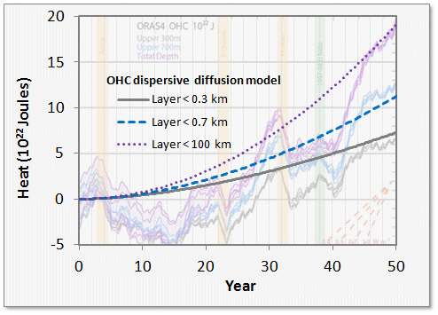
A good approximation is to assume the thermal forcing function started kicking in about 50 years ago, circa1960. We can then plot the equation for various values of the layer thickness, L, and a value of D of 3 cm^2/s.

Figure 2 : Thermal Dispersive Diffusion Model applied to the OHC data

Another view of the OHC includes the thermal mass of the non-ocean regions (see Figure 3). This data appears smoothed in comparison to the raw data of Figure 2.

Figure 3 :  Alternate view of growing ocean heat content. This also includes non-ocean.

In the latter figure, the agreement with the uncertainty-quantified theory is more striking. A single parameter, Hansen's effective diffusion coefficient D, along with the inferred external thermal forcing function is able to reproduce the temporal profile accurately.

The strength of this modeling approach is to lean on the maximum entropy principle to fill in the missing gaps where the variability in the numbers are uncertain.  In this case, the diffusion and ocean depths hold the uncertainty, and we use first-order phyiscs to do the rest.

Sanity Check

The following is a sanity check for the above formulation; providing essentially a homework assignment that a physics professor would hand out in class.

An application of Fick’’s Law is to approximate the amount of material that has diffused (with thermal diffusion coefficient D) at least a certain distance, x, over a time duration, t, by

$$ e^{\frac{-x}{\sqrt{Dt}}}= \frac{Q}{Q_0}$$

• For greater than 300 meters, Q/Q_0 is 13.5/20 read from Figure 1.
• For greater than 700 meters, Q/Q_0 is 7.5/20

Where Q_0=20 is the baseline for the total heat measured over all depths (i.e. between x=0 and x=infinite depth) reached at the current time. No heat will diffuse to infinite depths so at that point Q/Q_0 is 0/20.

First, we can check to see how close the value of L=sqrt(Dt) scales, by fitting the Q/Q_0 ratio at each depth..

• For x=300 meters, we get L=763
• For x=700 meters, we get L=713

These two are close enough to maintaining invariance that the Fick’’s law scaling relation holds and we can infer that the flow is by an effective diffusion, just as was surmised by Hansen et al in 1981.

We then use an average elapsed diffusion time of t=40 years and assume an average diffusion depth of 740, and D comes out to 4.5 cm^2/s.

Hansen in 1981 [2] used an estimated value of diffusion of 1 cm^2/s, which is within an order of magnitude of 4.5 cm^2/s

This is a scratch attempt at an approximate solution to the more general solution, which is the equivalent of generating an impulse function in the past and watching that evolve. The general solution which we formulated earlier involves a modulated forcing function and we compute the convolution against the thermal impulse response (i.e. Green’s function) and compare that against Figure 1 and Figure 2, and the full temporal profile.

Discussion

Reading Hansen and looking at the BTK paper’s results, we should note that nothing looks out of the ordinary for the OHC trending if we compare it to what conventional thermal physics would predict. The total heat absorbed by the ocean is within  range of that expected by a 3C doubling sensitivity. BTK has done the important step in determining the amount of total heat absorbed, which allows us to estimate the effective diffusion coefficient by evaluating how the heat contents modulate with depth.We add a maximum uncertainty modifier to the coefficient to model the disorder in diffusivity (some of it eddy diffusivity, some vertical, etc) and that allows us to match the temporal profile accurately.



References

[1]

M. A. Balmaseda, K. E. Trenberth, and E. Källén, “Distinctive climate signals in reanalysis of global ocean heat content,” Geophysical Research Letters, 2013.

[2]

J. Hansen, D. Johnson, A. Lacis, S. Lebedeff, P. Lee, D. Rind, and G. Russell, “Climate impact of increasing atmospheric carbon dioxide,” Science, vol. 213 (4511), pp. 957–966.
http://pubs.giss.nasa.gov/docs/1981/1981_Hansen_etal.pdf

Stochastic analysis of log sensitivity to CO2

Often both skeptics and non-skeptics of AGW will suggest that climate models and their simulations are becoming too unwieldy to handle.  Stochastic models of the climate are always an option to consider, as Marston points out in his paper "Looking for new problems to solve? Consider the climate", where he recommended to

"look at the sort of question a statistical description of the climate system would be expected to answer" [5] . 

It is no wonder that applying stochasticity is one of the grand challenges in science. In the past few years, DARPA put together a list of 23 mathematical challenges inspired by Hilbert's original list. Several of them feature large scale problems which would benefit from the stochastic angle that both Marston and David Mumford [4] have recommended:

• Mathematical Challenge 3: Capture and Harness Stochasticity in Nature
  Address David Mumford’s call for new mathematics for the 21st century. Develop methods that capture persistence in stochastic environments.  
• Mathematical Challenge 4: 21st Century Fluids Classical fluid dynamics and the Navier-Stokes Equation were extraordinarily successful in obtaining quantitative understanding of shock waves, turbulence and solitons, but new methods are needed to tackle complex fluids such as foams, suspensions, gels and liquid crystals.
• Mathematical Challenge 7: Occam’s Razor in Many Dimensions
  As data collection increases can we “do more with less” by finding lower bounds for sensing complexity in systems? This is related to questions about entropy maximization algorithms.
• Mathematical Challenge 20: Computation at Scale
  How can we develop asymptotics for a world with massively many degrees of freedom?

The common theme is one of reducing complexity, which is often at odds with the mindset of those convinced that only more detailed computations of complex models will accurately represent a system.

A representative phenomena of what stochastic processes are all about is the carbon cycle and the sequestering of CO2. Much work has gone into developing box models with various pathways leading to sequestering of industrial CO2. The response curve according to the BERN model [7] is series of damped exponentials showing the long term sequestering. Yet, by a more direct statistical interpretation of what is involved in the process of CO2 sequestration, we can model the adjustment time of CO2 decay by a dispersive diffusional model derived via maximum entropy principles.

$$ I(t) = \frac{1}{1+\sqrt{t/\tau}} $$

Figure 1 : Impulse response of atmospheric CO2 concentration due to excess carbon emission.

A main tenet of the AGW theory presupposes the evolution of excess CO2. The essential carbon-cycle physics says that the changing CO2 is naturally governed by a base level which changes with ambient temperature, but with an additional impulse response governed by a carbon stimulus, either natural (volcano) or artificial (man-made carbon). The latter process is described by a convolution, one of the bread and butter techniques of climate scientists:

$$CO_2(t,T) = CO_2(0,T) + \kappa \int_0^t C(\tau) I(t-\tau) d\tau $$

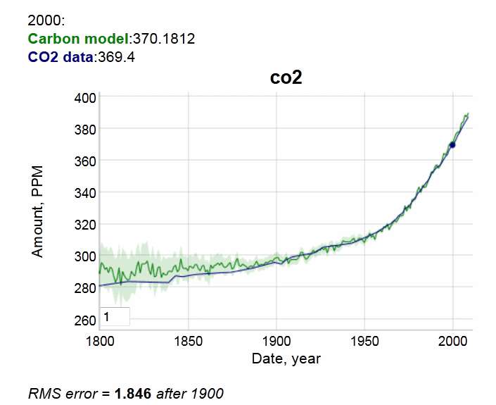
With the impulse response of Figure 1 convolved against the historical carbon outputs as archived at the CO2 Information Analysis Center, it matches the measured CO2 from the KNMI Climate Explorer with the following agreement:

Figure 2 : CO2 impulse response convolution

The match to the CO2 measurements is very good after the year 1900. No inexplicable loss of carbon to be seen. This is all explainable by diffusion kinetics into sequestration sites. Diffusional physics is so well understood that it is no longer arguable.

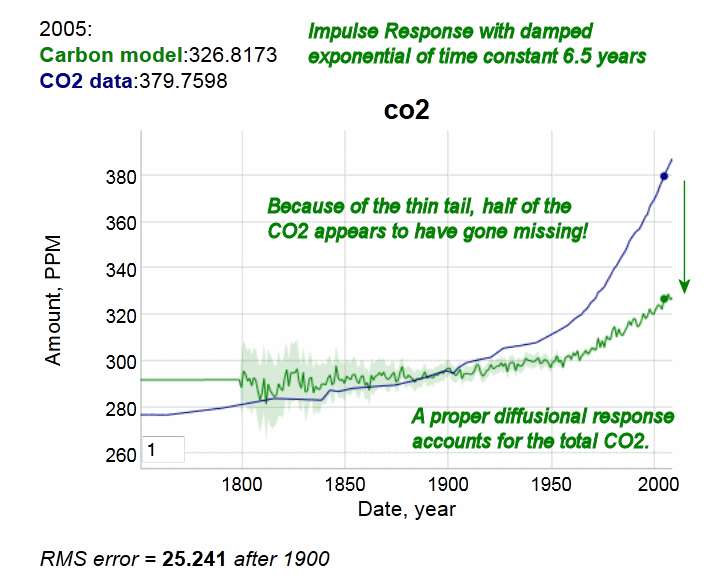
If on the other hand, you do this analysis incorrectly and use a naive damped exponential response ala Segalstad [1] and Salby [unpublished] and other contrarian climate scientists, you do end up apparently believing that half of the CO2 has gone missing. If that were indeed the case, this is what the response looks like, given the skeptics view of a short 6.5 year CO2 residence time:

Figure 3: Incorrect impulse response showing atmospheric CO2 deficit due to a short residence time.
This is clearly not observed in the data

The obvious conclusion is that if you don't do the statistical physics correctly, you end up with nonsense numbers.


Note that this does not contradict findings of the mainstream climate researchers, but it places our understanding on a potentially different footing, and one with potentially different insight.

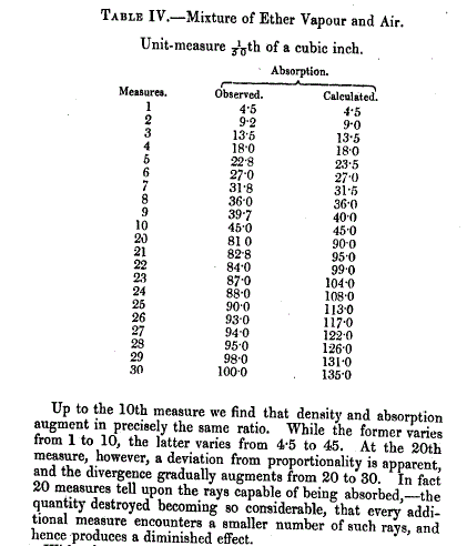
Consider next the sensitivity of temperature to the log of atmospheric CO2. In 1863, Tyndall discovered the properties of CO2 and other gases via an experimental apparatus [3];he noticed that light radiation absorption was linear up to a point but beyond that the absorptive properties of the gas showed a diminishing effect:

Figure 4: Tyndall's description of absorption of light rays by gases [6]

The non-linear nature derives from the logarithmic sensitivity of forcing to CO2 concentration. The way to understand this is to consider differential increases of gas concentration. In the test chamber experiment, this is just a differential increase in the length of the tube. The scattering cross-section is derived as a proportional increase to how much gas is already there so it integrates as the ratio of delta increase to the cumulative length of travel of the photon:

$$ \int_{L_0}^L \frac{dX}{X} = ln(\frac{L}{L_0}) \sim ln(\Delta{[CO_2]}) $$

So as the photon travels a length of tube, it gets progressively more difficult to increase the amount of scattering, not because it isn't physically possible but because the photon has had a large probability of being intercepted already as it makes its way out of the atmosphere. That generates the logarithmic sensitivity.

Note that the lower bound of the integral has to exist to prevent a singularity in the proportional increase. To represent this another way, we can say that there is a minimum length at which the absorption cross-section occurs.


$$ \int_{0}^L \frac{dX}{X_0+X} = ln(\frac{X_0+L}{X_0}) \sim ln(1+\Delta{[CO_2]}) $$


The analogy to the test chamber is the height of the atmosphere. The excess CO2 that we emit from burning fossil fuels increases the concentration at the top of the atmosphere, and that increases the length of the travel of the outgoing IR photons, and the same logarithmic sensitivity results. This is incorrectly labeled as saturating behavior, instead of an asymptotic logarithmic behavior.

I haven't seen this derived in this specific way but the math is high-school level integral calculus. The actual model used by Lacis and other climate scientists is to configure the cross-sections by compositing the atmosphere into layers or "slabs" and then propagating the interception of photons by CO2 by differential numerical calculations. In addition, there is a broadening of the spectral lines as concentration increases, contributing to the first order result of logarithmic sensitivity.  In general the more that the infrared parts of the photonic spectrum get trapped by CO2 and H20, the higher the temperature has to be to make up for the missing propagated wavelengths while not violating the earth's strict steady-state incoming/outgoing energy balance.

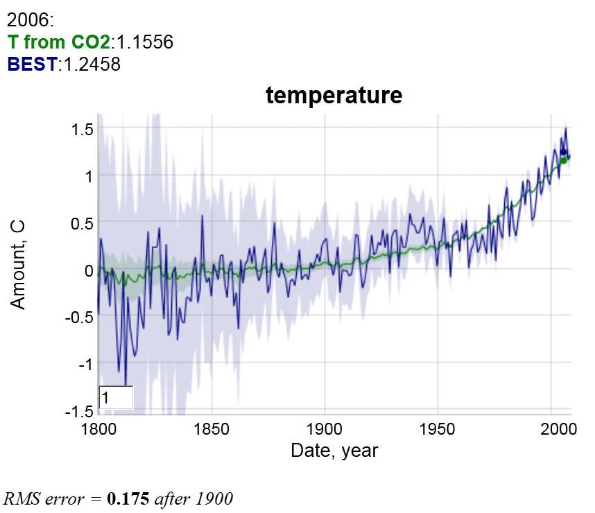
To get a sense of this logarithmic climate sensitivity, the temperature response is shown to the below  right for a 3°C sensitivity to CO2 doubling, mapped against the BEST land-based temperature record. Observe that trending temperature shifts are already observed in the early 20th century.

Figure 5:  CO2 model applied to AGW via a log sensitivity and
compared against the fast rsponse of BEST land-based records.

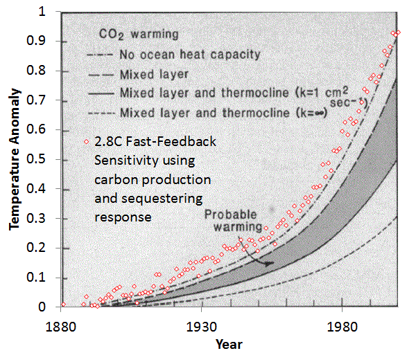
If we choose a 2.8°C sensitivity from Hansen's 1981 paper [2] and compare the above model to Hansen's projection, one can see that we are on the right track in duplicating his analysis.

Figure 6: Hansen's original model projection circa 1981 [2] and the 2.8C model used here.

Perhaps the only real departure from the model is a warming around 1940 not accounted for by CO2.  But even this is likely due to a stochastic characteristic in the form of noise riding along with the trend.. This noise could be volcanic disruptions or ocean upwelling fluctuations of a random nature,  which only requires the property that upward excursions match downward.

So if we consider the difference between the green line model and blue line data below:

Figure 7: Plot used for regression analysis.
Beyond 1900, the RMS error is less than 0.2 degrees

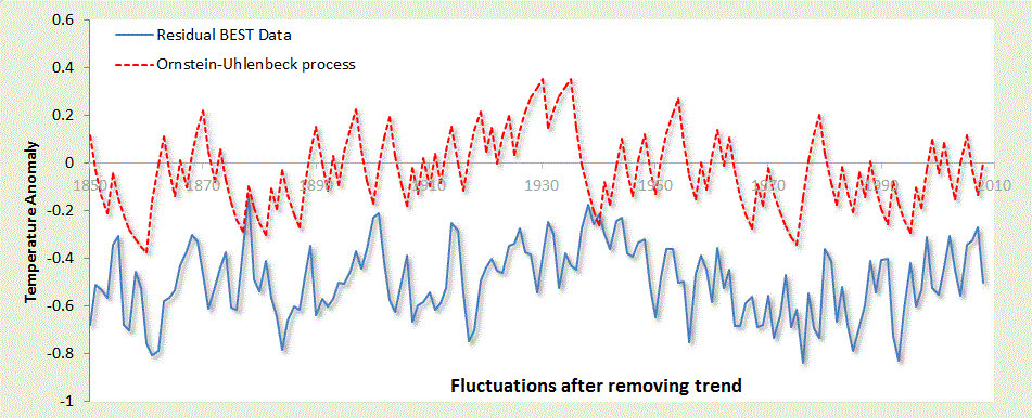
and take the model/data residuals over time, we get the following plot.

Figure 8: Regression difference between log sensitivity model and BEST data 

Note that the yearly excursions never exceed about 0.2°C from the underlying trend.  The dotted line red curve above the solid blue residual curve is an Ornstein-Uhlenbeck model (red noise) of a yearly random walk with a reversion-to-the-mean drag that prevents fluctuations beyond approximately 0.2°C.  At this kind of scale and considering the Markov process which will allow short-term fluctuations in the tenths of a degree, the bump of increased temperature in the 1940's is not a rare nor completely unlikely occurrence.

A red noise model on this scale can not accommodate both the short-term fluctuations and the large upward trend of the last 50 years. That is why the CO2-assisted warming is the true culprit, as evidenced by a completely stochastic analysis.

[EDIT]
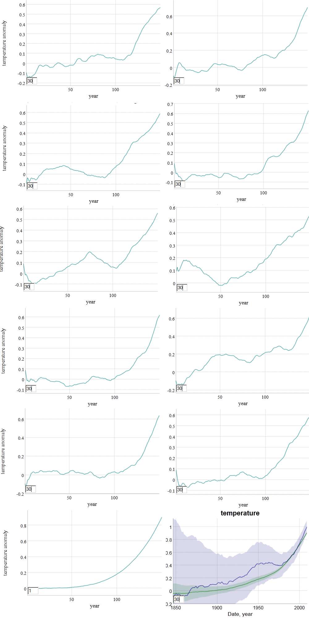
Here is a sequence of red noise time series (of approximately 0.2°C RMS excursion) placed on top of an accelerating monotonically warming temperature profile (the no-noise accelerating profile is in the lower left panel). The actual profile is shown in the lower right panel. An averaging window of 30 years is placed on the profiles to give an indication of where plateaus, pauses, and apparent cooling can occur.

Figure 9: Hypothetical red noise series placed on an accelerating warming curve.

"Noise riders" are people that look at time series and read too much into each fluctuation. The temptation to place too much emphasis on recent readings is strong but ultimately misguided. Dead reckoning models are built-in as a human intuition mechanism but don't serve us well in the face of noise.

The baseball analogy to the red noise of Figure 9 is the knuckle-ball pitcher. Being able to hit a knuckle-baller means that you have quick reflexes and an ability to suppress the dead reckoning urge.

R.A. Dickey's Cy Young Knuckleball Pitch (SOURCE)

References

[1]

T. V. Segalstad, “Carbon cycle modelling and the residence time of natural and anthropogenic atmospheric CO2,” BATE, R.(Ed., 1998): Global Warming, pp. 184–219, 1998.

[2]

J. Hansen, D. Johnson, A. Lacis, S. Lebedeff, P. Lee, D. Rind, and G. Russell, “Climate impact of increasing atmospheric carbon dioxide,” Science, 2l3, pp. 957–966.

[3]

A. A. Lacis, G. A. Schmidt, D. Rind, and R. A. Ruedy, “Atmospheric CO2: principal control knob governing Earth’s temperature,” Science, vol. 330, no. 6002, pp. 356–359, 2010.

[4]

D. Mumford, “The dawning of the age of stochasticity,” Mathematics: Frontiers and Perspectives, pp. 197–218, 2000.

[5]

B. Marston, “Looking for new problems to solve? Consider the climate,” Physics, vol. 4, p. 20, 2011.

[6] Tyndall, John, 1861. On the Absorption and Radiation of Heat by Gases and Vapours, and on the Physical Connection of Radiation, Absorption, and Conduction. 'Philosophical Magazine ser. 4, vol. 22, 169–94, 273–85.

[7] J. Golinski, “Parameters for tuning a simple carbon cycle model,” United Nations Framework Convention on Climate Change. [Online]. Available: http://unfccc.int/resource/brazil/carbon.html. [Accessed: 12-Mar-2013].

Spatial and Temporal Correlations of Wind

In terms of climate statistics, we always have more data than we know what to do with. The challenge is in reducing the data into meaningful bits of information which can be characterized and modeled succinctly.

So this is a case of where enough data exists that we can get an understanding of the spatial and temporal correlations of prevailing winds.

One source of data comes from measurements of winds at altitude, taken by jet airliners as part of their regular flight routes and then post-processed and analyzed[1]. This gives an indication of spatial correlation over a large dynamic range, stretching a little over three orders of magnitude.  Once collected, the post-processing involved applying an autocorrelation to the data over all spatial scales.  The power spectral density (PSD) is the Fourier transform of the autocorrelation, and that is shown in Figure 1 below, along with a suggested model achieving a good fit to the actual meridonal wind PSD.

Figure 1 : Zonal and Meridional wind speed PSD. The dashed line model fit works well apart from deviations near the noisy shorter wavelengths.

The chosen model is simply the PSD of an exponentially damped cosine autocorrelation (see [2] for examples in meteorology).

$$ C(x) = e^{-\alpha |x|} \cdot cos(\beta x) $$

The Fourier transform of this autocorrelation gives a PSD that is best described as a shifted Cauchy or Lorentzian profile.  In Figure 1, the shape is obvious as it shows a peak and then a concave-upward inflection following the peak.

$$ I(S_x) = \frac{\alpha}{(S_x-\beta)^2 + \alpha^2} $$

This specific profile is generated by a semi-Markovian process.  The "semi" part captures the periodic portion while the Markov contributes the memory for close-proximity coupling. Specifically, the Markov term is the alpha-factor damping which gives the overall 1/S^2 roll-off, while the beta-spatial shift indicates a semi-Markov ordering feature indicating some underlying longer-range spatial periodicity.

$$ \beta = 2 \pi/L = \text{1.3e-6 rad/m} $$
$$ \alpha  = \text{7.63e-7 rad/m} $$

This gives a weak periodicity of L=4833 km.   For a prevailing wind-stream of 30 MPH, this spans approximately 4 days of flow between a peak and a lull in wind speed. 

The spatial correlation intuitively leads to the concept of a temporal correlation in wind speed, and the question of whether this characteristic can be measured and contrasted to the spatial correlation.

For temporal correlation, I used the same data from the BPA which I had previously applied to a probability density function (PDF) analysis. 

Figure 2 : Temporal autocorrelation of wind speed

The temporal autocorrelation of the Roosevelt Island site shows some periodic fine structure. Using the Eureqa equation fitting software, I get the following empirical autocorrelation match.

$$ c(t)= 0.02934 \cdot sin(0.5012 - 1.626 t) + 0.01668 \cdot  cos(0.8645 + 6.203 t) + exp(-1.405 t) - 0.02134 \cdot sin(1.088 - 0.599 t) $$

The first and second terms are periodicities of 3.86 and 1 days, the latter easily explained by daily (diurnal) variations.  There is also a strong damping factor with a half-life less than a day. The last term is a 10 day period which generates a longer term modulation (and also has more uncertainty in its weighting).

The 3.86 day periodicity is likely due to a principle oscillation pattern in unstable meandering baroclinic Rossby waves as detected through a separate statistical analysis [3]

This demonstrates how the spatial correlation relates to the temporal correlation. As the tropospheric wave patterns propagate and disperse, they influence the local wind patterns.  These are quite subtle effects yet they can be detected and perhaps can be put to good use in battling the intermittency in wind power.

References

[1] G. Nastrom and K. S. Gage, “A climatology of atmospheric wavenumber spectra of wind and temperature observed by commercial aircraft,” Journal of the atmospheric sciences, vol. 42, no. 9, pp. 950–960, 1985.

[2] H. J. Thiebaux, “Experiments with correlation representations for objective analysis,” Monthly Weather Review, vol. 103, p. 617, 1975.

[3] H. Von Storch and F. W. Zwiers, Statistical analysis in climate research. Cambridge University Press, 2002.