Standard Atmosphere Model and Uncertainty in Entropy

(see this more recent derivation as well)

The lower atmosphere known as the troposphere is neither completely isentropic (constant entropy) nor completely isothermal (constant temperature).

An isentropic process will not exchange energy with the environment and therefore will maintain a constant entropy (also describing an adiabatic process).

If it was isothermal, all altitudes would be at the same temperature, realizing a disordered equilibrium state.This is maximum entropy as all the vertical layers are completely mixed.

Yet, when convective buoyancy results from evaporation, energy is exchanged up and down the column. And when green-house gases change the radiative properties of the layers, the temperature will also change to some degree.

So, how would we naively estimate what the standard atmospheric profile of such a disordered state would be?   The standard approach is to assume maximum uncertainty between the extremes of isentropic and isothermal conditions. This is essentially a mean estimate of half the entropy of the isothermal state, and a realization of Jaynes recommendation to assume maximum ignorance when confronted with the unknown.

We start with the differential representation

$$dH = V dp + T ds $$

Add in the ideal gas law assuming the universal gas constant and one mole.
$$ pv = RT $$

Add in change in enthalpy applying the specific heat capacity of air (at constant pressure).
$$dH = c_p dT$$

Substitute the above two into the first equation:
$$c_p dT =  \frac{RT}{p} dp  + T ds $$

Rearrange in integrable form
$$c_p \frac{dT}{T}  = \frac{R}{p} dp + ds $$

Integrate between the boundary conditions
$$c_p \cdot ln(\frac{T_1}{T_0} ) = R \cdot ln(\frac{p_1}{p_0}) + \Delta s $$

The average delta entropy change (loss) from a low temperature state to a high temperature state is:
$$ \Delta s = - \frac{1}{2}  c_p \cdot ln(\frac{T_1}{T_0} ) $$


The factor of 1/2 is critical because it represents an average entropy between zero entropy change and maximum entropy change.  So this is halfway in between an isentropic and an isothermal process (somewhere in the continuum of a polytropic process, categorized as a quasi-adiabatic process 1 < n < γ, where n is the polytropic index and γ is known as the adiabatic index or isentropic expansion factor or  heat capacity ratio).

Added Note: The loss or dispersion of energy is likely due to the molecules having to fight gravity to achieve a MaxEnt distribution as per the barometric formula. The average loss is half the potential energy of the barometric height (an average troposphere height) and this is reflected as half again of the dH kinetic heat term ½ CpΔT = mg ½ ΔZ.  This is a hypothesis to quantify the dispersed energy defined by the hidden states of  ΔS.

Substituting and rearranging: 
 $$ \frac{3}{2}  c_p \cdot ln(\frac{T_1}{T_0} ) = R \cdot ln(\frac{p_1}{p_0}) $$

which leads to the representation

$$ T_1 = T_0 \cdot (\frac{p_1}{p_0})^{R/{1.5 c_p}} $$

which only differs from the adiabatic process (below) in its modified power law (since n<γ it is a quasi-adiabatic process):

$$ T_1 = T_0 \cdot (\frac{p_1}{p_0})^{R/c_p} $$


The Standard Atmosphere model represents a typical barometric profile

The "Standard Atmosphere" is a hypothetical vertical distribution of atmospheric properties which, by international agreement, is roughly representative of year-round, mid-latitude conditions. Typical usages include altimeter calibrations and aircraft design and performance calculations. It should be recognized that actual conditions may vary considerably from this standard.

The most recent definition is the "US Standard Atmosphere, 1976" developed jointly by NOAA, NASA, and the USAF. It is an idealized, steady state representation of the earth's atmosphere from the surface to 1000 km, as it is assumed to exist during a period of moderate solar activity. The 1976 model is identical with the earlier 1962 standard up to 51 km, and with the International Civil Aviation Organization (ICAO) standard up to 32 km.

Using R = 287 J/K/kg, cp =1004 J/K/kg, we fit the equation that we derived above to the US Standard Atmosphere data set in the figure below:

Standard Atmosphere Model (circles) compared to average entropy derivation (line)

The correlation coefficient between the standard atmospheric model and the derived expression is very close to one, which means that the two models likely converge to the same reduced form.

How was the US Standard Atmosphere 1975 model chosen?  Was this empirically derived from measured temperature gradients (i.e. lapse rates) and barometric pressure profiles? Or was it estimated in an equivalent fashion to that derived here?

The globally averaged temperature gradient is 6.5 C/km, which is exactly g/(1.5cp). Compare this to the adiabatic gradient of 9.8 C/km = g/cp.

[EDITS below]

The exponent R/(1.5*cp) in the standard atmosphere derivation described above is
R/(1.5*cp) = 286.997/(1.5*1004.4) = α = 0.190493. Or, since cp = 7/2*R for an ideal diatomic gas, then R/(1.5*7/2*R) = α = 4/21 = 0.190476 .

Note from reference [1] that this same value of α is apparently a best fit to the data.

from O. G. Sorokhtin, G. V. Chilingarian, and N. O. Sorokhtin,
Evolution of Earth and its Climate: Birth, Life and Death of Earth. Elsevier Science, 2010.

What is the probability that a value fitted to empirically averaged data would match to a derived quantity to essentially 4 decimal places after rounding?  That would be quite a coincidence unless there is some fundamental maximum entropy truth (or perhaps the Virial theorem, K.E = ½  P.E.) hidden in the derived relation.

So essentially we have the T vs P relation for the US Standard Atmosphere as

$$ T_1 = T_0 \cdot (\frac{p_1}{p_0})^{4/21} $$

with very precise resolution.

Martin Tribus recounted his discussion with Shannon [2] :

from M. Tribus, “An engineer looks at Bayes,” in
Maximum-Entropy and Bayesian Methods in Science and Engineering, Springer, 1988.

I don't completely understand entropy either, but it seems to understand us and the world we live in. Entropy defined as dispersion of energy at a specific temperature often allows one to reason about the analysis through some intuitive notions.



References

[1]

O. G. Sorokhtin, G. V. Chilingarian, and N. O. Sorokhtin, Evolution of Earth and its Climate: Birth, Life and Death of Earth. Elsevier Science, 2010.

[2]

M. Tribus, “An engineer looks at Bayes,” in Maximum-Entropy and Bayesian Methods in Science and Engineering, Springer, 1988, pp. 31–52.

[UPDATE]

The lapse rate of temperature with altitude (i.e. gradient) is a characteristic that is easily measured for various advective planetary atmospheres.

If we refer to the polytropic factor 4/21 by f  then the lapse rate

$$ LR = f \cdot g \cdot MW / R $$

where g is the acceleration due to gravity on a planet, and MW is the average molar molecular weight of the atmospheric gas composition on the planet.  For the planets, Earth, Venus, Mars and the sun, the value of gravity and molecular weight are well characterized, with lapse rates documented in the references below.

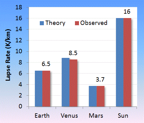
Observed lapse rate gathered for Mars [3,4], Venus [5,6,7], Sun [8].
Venus seems to have the greatest variability with altitude

Object	Theory	Observed	MW	g
Earth	6.506	6.5	28.96	9.807
Venus	8.827	8.5 ref [5]	43.44	8.87
Mars	3.703	3.7 ref [4]	43.56	3.711
Sun	16.01	16 ref [8]	2.55	274.0

The US Standard Atmosphere references the lapse rate as 6.5 while the International Civil Aviation Organization as 6.49. If we take the latter and adjust the composition of water vapor in the atmosphere to match, we come up with an 18% relative humidity at sea level extending to higher altitudes.

This change in humidity will cause a subtle change in lapse rate with global warming. As the relative humidity goes up with average temperature, the lapse rate will slightly decline, as water vapor is less dense than either molecular oxygen and nitrogen.  So this means that an increase in temperature at the top of the atmosphere due to excess GHG will be slightly compensated by a change in tropospheric height, i.e. that point where the barometric depth is equal to the optical depth. What magnitude of change this will make on surface temperature is worthy of further thought, but as has been known since Manabe, the shift toward heating is as shown in the figure below. Note how the profile shifts right (warmer) with additional greenhouse gases.

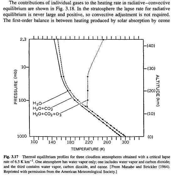
Change in lapse rate with atmospheric composition is subtle. The larger effect is in radiative trapping of heat thus leading to an overall temperature rise. Taken from [9]

The temperature of the earth is ultimately governed by the radiative physics of the greenhouse gases and the general application of Planck''s law.  Based on how the other planets behave (and even the sun) the thermodynamic aspects seem more set in stone.

Lapse Rate References 

[3]

R. Cess, V. Ramanathan, and T. Owen, “The Martian paleoclimate and enhanced atmospheric carbon dioxide,” Icarus, vol. 41, no. 1, pp. 159–165, 1980.

[4]

C. Fenselau, R. Caprioli, A. Nier, W. Hanson, A. Seiff, M. Mcelroy, N. Spencer, R. Duckett, T. Knight, and W. Cook, “Mass spectrometry in the exploration of Mars,” Journal of mass spectrometry, vol. 38, no. 1, pp. 1–10, 2003.

[5]

E. Palomba, “Venus surface properties from the analysis of the spectral slope@ 1.03-1.04 microns,” 2008.

[6]

A. Sinclair, J. P. Basart, D. Buhl, W. Gale, and M. Liwshitz, “Preliminary results of interferometric observations of Venus at 11.1-cm wavelength,” Radio Science, vol. 5, no. 2, pp. 347–354, 1970.

[7]

G. Fjeldbo, A. J. Kliore, and V. R. Eshleman, “The neutral atmosphere of Venus as studied with the Mariner V radio occultation experiments,” The Astronomical Journal, vol. 76, p. 123, 1971.

[8]

M. Molodenskii and L. Solov’ev, “Theory of equilibrium sunspots,” Astronomy Reports, vol. 37, pp. 83–87, 1993.

[9]

D. L. Hartmann, Global Physical Climatology. Elsevier Science, 1994.

[FINAL UPDATE]

CO2 is a polyatomic molecule and so (neglecting the vibrational modes) has 6 degrees of freedom (3 translation and 3 rotational) instead of the 5 (3 translational +2 rotational) of N2 and O2 in the gas phase.  Understanding that, we can adjust the polytropic factor from f = (1+5/2)*(3/2)=21/4=5.25 to f = (1+6/2)*3/2=6 for planets such as Venus and Mars.

Accessing more detailed atmospheric profiles of Venus, we can test the following thermo models for f=6, where T0 and P0 are the surface temperature and pressure.

Lapse Rate
$$ T_1 = T_0 \cdot (1 - z/(f z_0)) $$

Barometric Formula
$$ p_1 = p_0 \cdot (1 - z/(f z_0))^f $$

with
$$ z_0 = \frac{R T_0}{MW g} $$

P-T Curves

$$ p_1 = p_0 \cdot (\frac{T_1}{T_0})^f $$

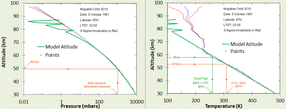
Barometric Formula Profile (left) and Lapse Rate Profile (right) as determined by the Magellan Venus probe. The model fit for f=6, and the estimated surface pressure is shown by the green line. T0 is the only adjustable parameter. The zig-zag green line is a deliberate momentary shift of f=6 to values of f=6.5, 6.7, and 6.85 to indicate how the profile is transitioning to a more isothermal regime at higher altitude.
Adapted from charts on Rich Townsend's MadStar web site:
http://www.astro.wisc.edu/~townsend/resource/teaching/diploma/venus-p.gif
http://www.astro.wisc.edu/~townsend/resource/teaching/diploma/venus-t.gif

The P-T profile which combines the Magellan data above with data provided on the "Atmosphere of Venus" Wikipedia page. The polytropic factor of 6 allows a good fit to the data to 3 orders of magnitude of atmospheric pressure. This includes the super-critical gas phase of CO2.

The lapse rate perhaps can be best understood by the following differential formulation

$$ \Delta E = m g \Delta z + c_p \Delta T $$

If 1/3 of the gravitational energy term is lost as convective kinetic energy, and cp=4R then

$$ \Delta E = 1/3 m g \Delta z = m g \Delta z + 4 R \Delta T $$
and this allows 2/3 of the gravitational energy to go through a quasi-adiabatic transition.

Whether this process describes precisely what happens (see Added Note in the first part of this post), it accurately matches the standard atmospheric profiles of Venus and Earth.  It also follows Mars well, but the variability is greater on Mars, as can be see seen in the figures below. The CO2-laden atmosphere of Mars is thin so the temperature varies quickly from day to night, and the polytropic profile is constantly adjusting itself to match the solar conditions.

Venus has a lower atmospheric lapse rate that is more uniform, while Mars shows higher fluctuations on top of the mean slope.  From http://www.lpl.arizona.edu/~showman/climate/venus-mars-pdflatex.pdf

Within the variability, Mars will show good agreement with the polytropic lapse rate =
(1/6)MW*g/R = (1/6)*43.56*3.711/8.314 = 3.24 K/km.
Chart adapted from

D. M. Hunten, “Composition and structure of planetary atmospheres,” Space Science Reviews, vol. 12, no. 5, pp. 539–599, 1971.

 

The Earth is described by the "Standard Atmosphere" polytropic profile which is shallower than the adiabatic.

Data from the Russian Venera probes to Venus, with model overlaid.  Adapted from

M. I. A. Marov and D. H. Grinspoon, The planet Venus. Yale University Press, 1998.

The Venus lapse rate accurately follows from LR= (1/6) g MW/R, where 6 is the polytropic factor. Adapted from:

V. Formisano, F. Angrilli, G. Arnold, S. Atreya, K. H. Baines, G. Bellucci, B. Bezard, F. Billebaud, D. Biondi, M. I. Blecka, L. Colangeli, L. Comolli, D. Crisp, M. D’Amore, T. Encrenaz, A. Ekonomov, F. Esposito, C. Fiorenza, S. Fonti, M. Giuranna, D. Grassi, B. Grieger, A. Grigoriev, J. Helbert, H. Hirsch, N. Ignatiev, A. Jurewicz, I. Khatuntsev, S. Lebonnois, E. Lellouch, A. Mattana, A. Maturilli, E. Mencarelli, M. Michalska, J. Lopez Moreno, B. Moshkin, F. Nespoli, Y. Nikolsky, F. Nuccilli, P. Orleanski, E. Palomba, G. Piccioni, M. Rataj, G. Rinaldi, M. Rossi, B. Saggin, D. Stam, D. Titov, G. Visconti, and L. Zasova, “The planetary fourier spectrometer (PFS) onboard the European Venus Express mission,” Planetary and Space Science, vol. 54, no. 13–14, pp. 1298–1314, Nov. 2006.

Final Caveat: Not all planets follow this polytropic quasi-adiabatic profile.  The "big planets" of our solar system seem to follow the dry adiabatic very well at low atmospheric altitudes, see figure below. All of these consist mainly of H2 and a scattering of Helium (mono-atomic gas with Cp=5/2R) and so are slightly below 7/2R for a value of cp. Convective losses don't seem to play a role on these planets, in contrast to the sun, which is special in that the radiative temperature gradient can easily exceed the adiabatic lapse rate. In this case, the sun's atmosphere becomes collectively unstable and convective energy transport takes over (see T. I. Gombosi, Physics of the space environment. Springer, 1998, p.217).

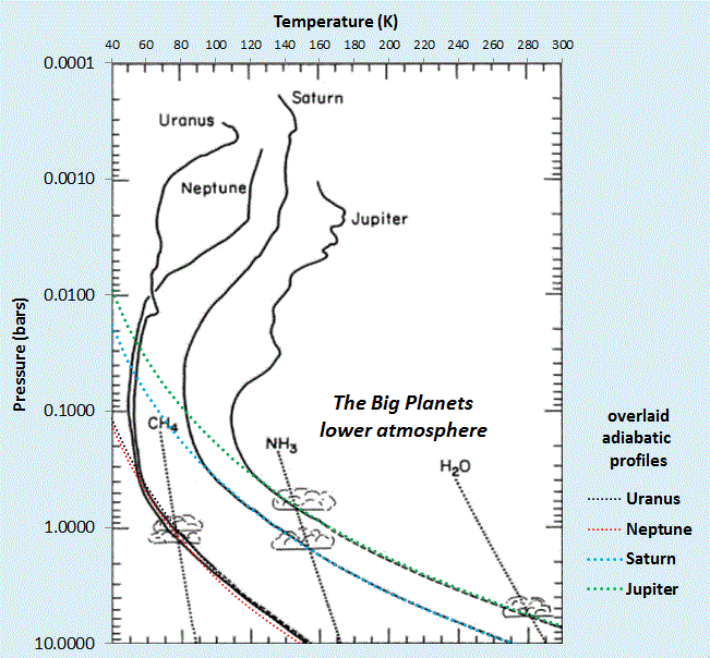
The "Big Planets" of our solar system have lower atmospheres that follow the adiabatic profiles closely.
Adapted from :
L. A. McFadden, P. Weissman, and T. Johnson, Encyclopedia of the Solar System. Elsevier Science, 2006.

All the planets (Venus not shown) follow either polytropic or adiabatic P-T profiles in the lower atmosphere.
Adapted from :

F. Bagenal, “Planetary Atmospheres ASTR3720 course notes.” [Online]. Available: http://lasp.colorado.edu/~bagenal/3720/index.html. [Accessed: 01-May-2013].

Climate Sensitivity and the 33C Discrepancy

The connection between greenhouse gases such as CO2  and climate change is solid. The global land temperature record is easily on track for a 3° C swing due to a doubling of CO2 levels; this also happens to be the consensus mean for climate sensitivity over a set of peer-reviewed models.

The breakdown of the 3°C doubling is that it is equal parts due to CO2 doubling, water vapor (which comes along for a ride), and a set of miscellaneous positive feedbacks

"If Earth were a blackbody without climate feedbacks the equilibrium response to 4 W/m2 forcing would be about 1.2°C (Hansen et al., 1981, 1984; Lacis et al., 2010), implying that the net effect of all fast feedbacks is to amplify the equilibrium climate response by a factor 2.5. GISS climate models suggest that water vapor and sea ice feedbacks together amplify the sensitivity from 1.2°C to 2-2.5°C. The further amplification to 3°C is the net effect of all other processes, with the most important ones probably being aerosols, clouds, and their interactions. "

 J. E. Hansen and M. Sato, “Paleoclimate implications for human-made climate change,” Climate Change, pp. 21–47, 2012. 

All the pieces to the climate change puzzle are interlocking. Every new piece of evidence has to be consistent with prior understanding, otherwise it weakens the consensus view. I have not been very successfull at finding any real holes in the GHG AGW argument myself. That is likely more do to my lack of detailed knowledge of the intricacies of the models, but it doesn't prevent me from trying other angles. For example, in lieu of my finding any breakthrough debunking arguments, I seek to find simplifications in the overall argument.

This post describes an interesting derivation that ties together the climate sensitivity of CO2 and water vapor along with the 33° C discrepancy between the no-GHG earth and our current average global temperature.

We start with an assumption that the baseline radiatively steady-state temperature is T0 and the temperature raises due to the climate sensitivity:
$$ T = T_0 + \alpha \log(C/C_0) $$
We assume that the second term is mainly due to water vapor, catalyzed by introduction of CO2. This is enough to raise the temperature from a ground-state snowball earth which would occur as the water would normally condense out at 255° K. Thereafter, the water vapor undergoes a bootstrapping process, whereby a fraction of the outgassed vapor serves to feed on itself, and through the GHG process raises the temperature further, leading to more outgassing.

The log dependence of water vapor concentration, C, on temperature, T, reflects the doubling sensitivity of a GHG. Water vapor works much like CO2 in this regard, only that it needs a boost from a non-condensing gas to sustain its elevated concentration.

Next, we assume the outgassing of water vapor follows the Clausius-Clapeyron activation relation, whereby the partial pressure is activated by a Boltzmann factor with an activation energy corresponding to the heat of vaporization.
$$ H = 0.42\:{ eV} = 4873\:{ Kelvins} $$
Then
$$ C/C_0 = \beta e^{-H/T} $$
We can make the assumption that the temperature, T, reaches a steady-state such that the positive feedback limits its extent as the Boltzmann acts as a rather weak feedback term. (This is not runaway warming we are talking about)

When we make the algebraic substitution for C/C0 in the first equation.
$$ T = T_0 + \alpha \log(\beta e^{-H/T}) $$
Because of the log(exp(X))=X identity this reduces to:
$$ T = T_0 + \alpha \log(\beta) - \alpha H / T $$
In terms of solution space, this is a quadratic with respect to temperature. For real valuations, we have a low temperature and high temperature solution.

Graphically, the intersection points look like the following.

Figure 1: Graphical solution to constrained positive feedback.
The red dots show the intersection points.

Mapping this to the real process that is occurring, the low T point likely corresponds to the no-GHG temperature of 255° K, while the high T point is intuitively the steady-state temperature of 289° K. In other words, the gap between the two intersection points is 33° C.
The quadratic equation is
$$ T^2 - (T_0 + \alpha \beta) T - \alpha H $$
with solution
$$ T=\frac{-\gamma\pm\sqrt{\gamma^2-4\alpha H}}{2} $$
where
$$ \gamma = T_0 + \alpha \log(\beta) $$
Safely assuming that the cold and hot solutions are symmetric about the midway point (255+289)/2 :
$$ \Delta T = \pm \sqrt{\gamma^2 - 4 \alpha H}/2 = \pm 16.5° C$$
where
$$ \gamma = T_{low} + T_{high} $$
We can now invert to determine alpha:
$$ \alpha = \frac {\gamma^2 -{2 \Delta T}^2}{4 H} $$
Inserting the values for the 3 fixed values:
$$ \alpha = 15.1° C $$
The climate sensitivity for a doubling of water vapor is
$$ 10.5° C = 15.1 log(2) $$
Finally, we can calculate how much a CO2-induced temperature change will trigger a corresponding rise in water vapor-induced temperature, i.e. it acts as the control knob as Lacis phrased it.

From the differential Clausius-Clapeyron $$ dC/C = {H/T^2} dT $$
with the standard dT for CO2 doubling given by Lacis [1] of 1.23°C. Then dC/C = 0.072 at T=289°K, which gives a sensitivity
$$ \alpha \log(1+dC/C) = 1.05° C $$
for the water vapor rise carried along by the CO2 doubling.
To get to the 3.0° C value we add together 1.23° C from CO2, 1.05° from H20, and approximately 0.7° C from other GHGs (see The NOAA Annual Greenhouse Gas Index) and albedo positive feedbacks.


Comparing to the Berkeley BEST land-based temperature values  with two different sensitivities, one can see how well the consensus value tracks the historical data.

Figure 2: Consensus CO2 GHG model against historical temperature data.
Lower curve is sensitivity of 3°C for a doubling of CO2

---

[1]  A. A. Lacis, G. A. Schmidt, D. Rind, and R. A. Ruedy, “Atmospheric CO2: principal control knob governing Earth’s temperature,” Science, vol. 330, no. 6002, pp. 356–359, 2010.

Climate Change and the Energy Problem

A recent book by David Goodstein called "Climate Change and the Energy Problem: physical science and economics perspective" has slipped under the radar. Goodstein is a professor of physics at CalTech and a disciple of Richard Feynman, the AGW skeptics' favorite quote-machine.

This is the follow-on to Goodstein's earlier book "Out of Gas" that ties together the hydrocarbon depletion challenge with the climate change problem. In interviews, Goodstein agrees that climate denialism, at its root, is a desire not to face the energy problem. He says that the people seriously working on peak oil are not at the margins but are at the forefront of change.

Goodstein has serious credentials, and is one of the top thermodynamics and condensed matter physicists in the world. He treats the AGW problem as obvious:

"Fortunately for us, that is not all there is to it. If the average surface temperature of the Earth were 0°F. we probably would not have been here. The Earth has a gaseous atmosphere, largely transparent to sunlight, but nearly opaque to the planet's infrared radiation. The blanket of atmosphere traps and reradiates part of the heat that the Earth is trying to radiate away. The books remain balanced, with the atmosphere radiating into space the sonic amount of energy the Earth receives, but also radiating heat back to the Earth's surface, warming it to a comfortable average temperature of 57°F. That is what is known as the greenhouse effect. Without the greenhouse effect and the global warming that results, we probably would not be alive. "

And Goodstein is also formidable when it comes to dealing with crackpots. His true skeptical credentials are revealed in his book "On Fact and Fraud: Cautionary Tales from the Front Lines of Science". This is a fascinating read as it deals with the Pons/Fleischmann cold fusion debacle as well as the Schon affair which I am very familiar with.

The interview linked above is good. Goodstein sounds like a Brooklynite and delivers answers to the questions in short, no-nonsense  replies.  The only chuckle that I heard was when the interviewer remarked that coal-power was not used to mine and transport the coal. 

Throughout Goodman stresses the significance of liquid fuel,  revealing the difficulty in boot-strapping the lower-grade forms of fossil fuels. 

The Peak Warmers

The question is whether we can use use solar energy to process all the oil shale or whether this is mind boggling in scope. If you apply your intuition, consider what it will take to collect solar energy in the form of electricity and then use that electricity to (1) dig out that shale and process it or (2) in situ process the shale via heat and refine something approaching a liquid from the kerogen. And then to deliver it to its destination.

The fear is that is is also possible that we will figure out how to bootstrap the entire oil shale process, whereby we use the energy from the oil shale to "extract itself". That obviously is the case with crude oil, as all the energy going to extract the oil comes from oil-powered machinery and transportation.

I think that occurred also in the early days of coal extraction, but at some point the returns start to diminish. Remember that coal is barely refined before it is used.

That is the most frightening prospect in all this, that well more than half of the hydrocarbon energy becomes a kind of waste heat. This is energy that isn't necessarily wasted because it is used for processing (see the concepts of EROEI and emergy), but that is essentially wasted as overhead and not directly contributing to propelling the world's economy.

Suddenly 80+ million barrels a day turns into 200 million equivalent barrels because 120 million barrels is used to process the 80. And that is just to keep in place with the needs of a growing global economy.

That leads into Pierrehumbert's reference to the Red Queen scenario in his Slate article. The Red Queen is about running faster just to keep in place. But oil shale makes it worse, as it turns the Red Queen into a voracious cannibal, while eating any seed corn and feedstock we have left.

Pierrehumbert states at the end of his article "Temporarily cheap and abundant gas buys us some respite—which we should be using to put decarbonized energy systems in place."

Can we be patient with the use of solar energy or will the second law be insurmountable?


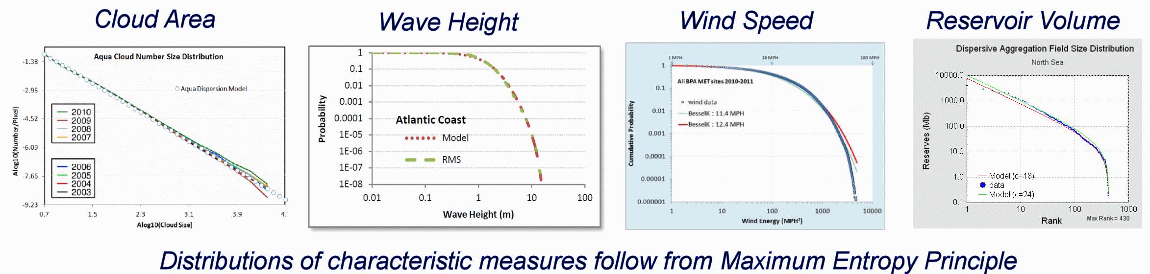
The dispersion in wind speeds already follows the second law of thermodynamics. Given a mean wind speed, applying the maximum entropy principle results in the observed variability.
Same goes for aquatic wave height variation.
Same goes for the areal coverage of clouds, which in turn will periodically obscure the sunlight.

Here is a pic that illustrates how nature follows the Maximum Entropy Principle:

click to magnify

That is the hurdle in dealing with the second law from a source perspective. Everything is variable because nature tries to fill up all available states, mixing the low-likelihood high energy states with the higher-likelihood low-energy states.

Through a freak of nature, our crude oil supplies were given to us in a very low entropy highly ordered configuration. But even there, the second law applies, as the volume distribution of reservoir sizes follows the maximum entropy principle. The tails in the distribution ultimately become the dispersed pockets we are now essentially mining. We used up all the higher-energy configurations first, and now are left with the lower energy configurations.

The other hurdle is one of entropic losses as we convert one energy form to another, which is needed to do all the processing of oil shales, etc.

So not only does entropy barely let us in, but it kicks our butt as we try to get out the door.
The objective really should be in how to sustainably harness the stochasticity in nature and not try to outdo it and burn ourselves into oblivion.

Patience is the key. Collect the highly dispersed energy sources from the sun, wind, etc. into a more concentrated form and then work with that. After all, isn't that how oil reservoirs formed in the first place?

However, growing economies have no room for patience.

This innocuous comment of mine was deleted from The Oil Drum today. Never can understand why they decide to delete what they do.

On the other hand, the blogger Willis Eschenbach has to be the most wrong-headed blowhard that has ever graced the internet.  If you ever want to do science properly, read what he writes, try to figure out how he approaches science, and then do the exact opposite. Oh, and think a little bit, not spew every idea that comes into your head, because the sycophantic followers that you will attract will not be able to discriminate between garbage and something worthwhile.

This is how inflated a sense of worth he possesses:

"Here on WUWT, I put out my scientific ideas up in the public forum as clearly as I can explain them, and I hand around the hammers, and people do their best to demolish my claims. That is science at its finest, nothing hidden, everything visible, all the relevant data and code available for any reader to either check my work, or to tear it to shreds, or to pick it up and take it further.
This gradual scientific migration to the web is well underway, moved forwards by things like journals with open review, and by other blogs. Science done in the dark by a few learned boffins is already dead in the 21st century, the practitioners just didn’t notice when they ran past their use-by dates, and as a result that dark corner of the scientific world is populated more and more by zombies. Zombies with PhD’s to be sure, but zombies nonetheless, everyone else is emerging into the light. Good news is, it’s somewhat of a self-limiting phenomenon, the best authors say that zombies can’t reproduce …"

The Luke Oilers

In the climate science world, those who side with consensus science and agree that anthropogenic global warming is real are at a minimum referred to as "lukewarmers".
These people may not be as rabid as the true-believers, yet they don't dismiss the scientific theory and evidence as do the so-called "climate deniers".

I ran across a similar type of minimal acceptance, though very muted and disguised, when I participated in a blog comment discussion at Climate Etc.  The top-level post concerned Maugeri's wrong-headed analysis and conclusion of near-cornucopian oil availability.

In the ensuing discussion, it was clear that the climate skeptics, who would otherwise not admit that Peak Oil was real, would nevertheless continue to push  alternatives such as nuclear and unconventional oil, and suggest that BAU could continue.  This contradiction pointed to the fact that they implicitly agree in the Peak Oil concept while denying that the progressives and technocrats (such as Hubbert) were correct in their overall assessment.

I suggest these implicit Peak Oil believers need to be referred to as "luke-oilers", distinct from the explicit Peak Oilers.  To be a luke-oiler, all it takes for you is to admit that the Bakken or the Tar Sands or nuclear will meet our future energy needs. Its actually not that high a bar that you have to clear to be a luke-oiler, but it wasn't high for a lukewarmer either -- just an admission to the facts on the the ground. The earth is warming due to man, and the oil is depleting due to man.

---

At the cross-roads of peak oil and climate science we see a world of dogs and cats, living together. On occasion this gets stirred up as in this Slate opinion piece by noted climate scientist and atmospheric physicist Raymond T. Pierrehumbert. The title is 'The Myth of “Saudi America”: Straight talk from geologists about our new era of oil abundance.'

In this piece Pierrehumbert discusses the issue of Bakken oil and acknowledges Rune Likvern's analysis of Red Queen behavior in shale oil.  At the end, he suggests a kind of "No Regrets" policy in that we move rapidly toward alternatives to oil, using the oil that we have right now to solve both the predicaments of oil depletion and AGW.